One-way ANOVA: Test Statistic

Chapter 10: Analysis of Variance: One-way Analysis of Variance

One-way ANOVA: Test Statistic

Once the hypotheses of a one-way ANOVA have been constructed and random samples have been drawn from the different populations, the next step of the procedure is the calculation of the test statistic that will determine whether or not the null hypothesis of equal population means is rejected.

The calculation of the test statistic starts by using the sample data to get an estimate of the population means #\mu_i# and the grand population mean #\mu#.

Sample Mean and Grand Sample Mean
Let #Y_{ij}# denote the measured value of the outcome variable for the #j#th observation in the sample corresponding to level #i# of the factor.

To get an estimate of the population means #\mu_i#, we calculate the sample means #\bar{Y}_i#:
\[\bar{Y}_i = \cfrac{\displaystyle\sum^{n_i}_{j=1}Y_{ij}}{n_i}\]

To get an estimate of grand population mean #\mu#, we calculate the grand sample mean #\bar{Y}#:
\[\begin{array}{rcl}
\bar{Y} &=& \cfrac{\displaystyle\sum^I_{i=1}\displaystyle\sum^{n_i}_{j=1}Y_{ij}}{N} \\\\
&=& \cfrac{\displaystyle\sum^I_{i=1}n_i\bar{Y}_i}{N}
\end{array}\]

In a study on the effects of sleep deprivation on driving ability, #N = 15# participants were recruited and randomly assigned to one of #3# groups: no sleep deprivation (group 1), 24 hours of sleep deprivation (group 2), or 48 hours of sleep deprivation (group 3).

Subsequently, the participants were put in a simulator and tested on various driving abilities, while the researchers kept track of the number of mistakes made.

Here the number of mistakes made is the outcome variable #Y# and sleep deprivation is the factor with #I=3# levels.

The hypotheses that are being tested are:
\[\begin{array}{rcl}
H_0&:& \mu_{0\,\text{hours}} = \mu_{24\,\text{hours}} = \mu_{48\,\text{hours}}\\
&&\text{(All population means are equal, i.e., sleep deprivation has no effect on the number of}\\
&&\text{errors made.)}\\\\
H_a&:& \mu_{0\,\text{hours}} \neq \mu_{24\,\text{hours}} \,\text{ or }\, \mu_{0\,\text{hours}} \neq \mu_{48\,\text{hours}}\,\text{ or }\, \mu_{24\,\text{hours}} \neq \mu_{48\,\text{hours}}\\
&&\text{(At least one population mean differs from another population mean, i.e., sleep deprivation}\\
&&\text{does have an effect on the number of errors made.)}
\end{array}\]
The results of the experiment are summarized in the following table:

	Hours of sleep deprivation
	Group 1 (0 hours)	Group 2 (24 hours)	Group 3 (48 hours)
	2	8	20
	3	7	12
	1	4	10
	2	10	24
	1	6	9
Sample mean (#\bar{Y}_i)#:	2	7	15	Grand sample mean (#\bar{Y}#): 8

The calculations of the sample means are:
\[\begin{array}{rcl}
\bar{Y}_i &=& \cfrac{\displaystyle\sum^{n_i}_{j=1}Y_{ij}}{n_i}\\\\
\bar{Y}_1 &=& \cfrac{2+5+0+2+1}{5}=2\\\\
\bar{Y}_2 &=& \cfrac{8+7+4+10+6}{5}=7\\\\
\bar{Y}_3&=& \cfrac{15+12+14+21+13}{5}=15\\\\
\end{array}\] And the calculation of grand sample mean is:
\[\begin{array}{rcl}
\bar{Y} &=& \cfrac{\displaystyle\sum^I_{i=1}n_i\bar{Y}_i}{N}\\\\
&=& \cfrac{(5\cdot2) + (5\cdot7) + (5\cdot15)}{15} = 8
\end{array}\]

Once the sample means and the grand sample mean are known, the next step is to use these means to calculate two types of variances: the between-sample variance and the within-sample variance.

One-way ANOVA Test Statistic and Null Distribution
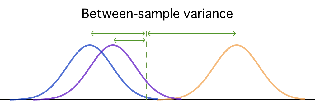
The between-sample variance estimates the differences between populations and is calculated by comparing the mean of each sample to the grand mean of the overall sample.

Between-sample variance has two possible sources:

Treatment effect. A treatment effect occurs when the null hypothesis is false and at least one of the population means differs from the others. If this is true, then we would expect the samples drawn from these populations to have different means as well.
Random error. Even if the null hypothesis is true and all population means are equal, we would still expect there to be some differences between samples. After all, each sample is made up out of different individuals, which should result in at least some sample-to-sample variability.

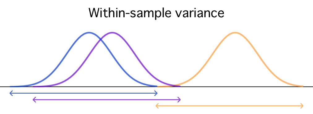
The within-sample variance is calculated by comparing the observations within each sample to their respective sample mean.

Since all individuals within a sample are drawn from the same population, the only source of within-sample variance is random error.

The test statistic #F# of a one-way ANOVA is defined as the ratio of the between-sample variance to the within-sample variance:
\[F=\cfrac{\text{between-sample variance}}{\text{within-sample variance}}\] If we express the two types of variance in terms of their possible sources, then the definition of the #F#-statistic becomes:
\[F=\,\cfrac{\text{Treatment effect} + \text{Random error}}{\text{Random error}}\] Depending on whether or not the null hypothesis is true, we expect to see the different values for this #F#-statistic:

If the null hypothesis is true and a treatment effect does not exist, then the between-sample differences found are entirely attributable to chance. In that case, both the between-sample variance and the within-sample variance are only measuring random error, and we should find an #F#-statistic roughly equal to #1#.
\[F=\,\cfrac{\text{Treatment effect} + \text{Random error}}{\text{Random error}}=\,\cfrac{0 + \text{Random error}}{\text{Random error}} \approx 1\]
If, on the other hand, the null hypothesis is false and a treatment effect does exist, then the between-sample variance should be relatively large compared to the within-sample variance, and we should find an #F#-statistic noticeably larger than #1#.
\[F=\,\cfrac{\text{Treatment effect} + \text{Random error}}{\text{Random error}}=\,\cfrac{\text{Treatment effect}}{\text{Random error}} + \,\cfrac{\text{Random error}}{\text{Random error}} \gg 1\]

If the assumptions of the ANOVA are satisfied, the #F#-statistic follows the #F#-distribution with #df_{model} = I-1# degrees of freedom in the numerator and #df_{error} = N-I# degrees of freedom in the denominator.

All #F#-distributions are positively skewed and the critical region of an ANOVA will always be located in the right tail of the distribution.

The #p#-value of the test is computed as #\mathbb{P}(F \geq f)#, where #f# is the observed value of #F#. A small #p#-value is interpreted as strong evidence against the null hypothesis and thus supports the conclusion that the population means #\mu_i# are not all the same, i.e., that the factor has a significant effect on the outcome variable.

Calculation of the one-way ANOVA Test Statistic
Note: In practice, the calculation of the #F#-statistic and its corresponding #p#-value is best left to statistical software, which typically summarizes its findings in an ANOVA table (shown below).

The calculations of the between-sample variance and the within-sample variance are basically exactly the same as the calculation of the 'regular' sample variance. Recall that this is done by completing the following steps:

For each observation #X_i# in the sample, calculate its deviation from the sample mean #\bar{X}#.
\[X_i-\bar{X}\]
Square each deviation to prevent positive and negative deviations from canceling each other.
\[(X_i-\bar{X})^2\]
Sum the squared deviations to create a measure of the total variability in the sample, called the sum of squares #SS#.
\[SS = \displaystyle\sum_{i=1}^n(X_i-\bar{X})^2\]
Divide the sum of squares by the number of scores in the sample (minus #1#) to create a measure of the average variability per score, called the mean squared deviation or sample variance #s^2#.
\[s^2 = \cfrac{\displaystyle\sum_{i=1}^n(X_i-\bar{X})^2}{n-1}\]

If this sounds at all unfamiliar, we would advise you to review these steps in more detail before proceeding.

The calculation of the between-sample and within-sample variances very closely mirrors the process outlined above. In both cases, we start by calculating a measure of the total variability called a sum of squares.

The total variability of the sample means #\bar{Y}_i# around the grand sample mean #\bar{Y}#, i.e. the between-sample variability, is measured by a quantity called the model sum of squares (#SS_{model}#), which is given by:
\[SS_{model} = \displaystyle\sum^I_{i=1}n_i\Big(\bar{Y}_i - \bar{Y}\Big)^2\]

The total variability of the observations in each sample #Y_{ij}# around their sample mean #\bar{Y}_i#, i.e. the within-sample variability, is measured by a quantity called the error sum of squares (#SS_{error}#), which is given by:
\[SS_{error} = \displaystyle\sum^I_{i=1}\displaystyle\sum^{n_i}_{j=1}\Big(Y_{ij} - \bar{Y}_i\Big)^2\]

However, because both these measures are sums, their size heavily depends on the number of values used in their calculation. Specifically, the size of the model sum of squares depends on the number of samples that are being compared, and the error sum of squares depends on the total number of observations in those samples.

To eliminate this bias, we calculate an average sum of squares, known as a mean square.

The model sum of squares is divided by the model degrees of freedom (#df_{model} = I - 1#) to calculate the model mean square (#MS_{model}#):
\[MS_{model} = \cfrac{SS_{model}}{I - 1}\]

And the error sum of squares is divided by the error degrees of freedom (#df_{error} = N - I\,#) to calculate the error mean square (#MS_{error}#):
\[MS_{error} = \cfrac{SS_{error}}{N - I}\]

Finally, the test statistic #F# is calculated as the ratio of the model mean square to the error mean square:\[F = \cfrac{MS_{model}}{MS_{error}}\]

The results of an ANOVA are typically summarized in an ANOVA table:

ANOVA
Outcome variable
	Sum of Squares	df	Mean Square	F	Sig.
Model	\[\displaystyle\sum^I_{i=1}n_i\Big(\bar{Y}_i - \bar{Y}\Big)^2\]	\[I-1\]	\[\cfrac{SS_{model}}{I - 1}\]	\[\cfrac{MS_{model}}{MS_{error}}\]	\[\mathbb{P}(F \geq f)\]
Error	\[\displaystyle\sum^I_{i=1}\displaystyle\sum^{n_i}_{j=1}\Big(Y_{ij} - \bar{Y}_i\Big)^2\]	\[N-I\]	\[\cfrac{SS_{error}}{N - I}\]

An example of an ANOVA table generated by #\mathrm{SPSS}# can be seen below.

ANOVA
Happiness
	Sum of Squares	df	Mean Square	F	Sig.
Between Groups	0.192	3	0.064	1.879	0.142
Within Groups	2.113	62	0.034
Total	2.305	65

Based on this ANOVA table, we would not reject the null hypothesis at the #\alpha = 0.01# level of significance, since #p > .01#, and conclude that the population means across the different levels of the factor are all equal.

An example of an ANOVA table generated by #\mathrm{R}# can be seen below.

               Df Sum Sq Mean Sq F value Pr(>F)    
IV              3     65   21.72     5.8  0.002 **
Residuals      36    135    3.74                   
---
Signif. codes:  0 ‘***’ 0.001 ‘**’ 0.01 ‘*’ 0.05 ‘.’ 0.1 ‘ ’ 1

Based on this ANOVA table, we would reject the null hypothesis at the #\alpha = 0.01# level of significance, since #p < .01#, and conclude that the population means across the different levels of the factor are not all equal.