One-way ANOVA: Hypotheses and Logic

Chapter 10: Analysis of Variance: One-way Analysis of Variance

One-way ANOVA: Hypotheses and Logic

One-way ANOVA Purpose
The one-way Analysis of Variance procedure is used to test whether the mean values of a continuous variable differ across three or more populations defined by a single categorical factor.

In general, the factor has #I# levels, and the population mean for the outcome variable #Y# for level #i# is #\mu_i#, for #i = 1,...,I#.

One-way ANOVA Hypotheses
The hypotheses of a one-way ANOVA are as follows:

#H_0#	#:#	The population mean for the outcome variable is the same across all #I# populations. #(\mu_1 = \mu_2 = \dots = \mu_I)#
		# \ #
#H_1#	#:#	At least one population mean differs from another population mean. #(\mu _i \neq \mu _j# for at least one pair of levels #(i,j))#

Take note that the alternative hypothesis of a one-way ANOVA does not specify which of the population means are supposed to be different. Consequently, the result of a one-way ANOVA only tells you if there is a significant difference between the means, but not which means differ.

If the null hypothesis of a one-way ANOVA is rejected, then a post hoc test should be run to determine which of the population means are different.

Consider a one-factor experiment in which the outcome variable is the change in systolic blood pressure, and the factor is the type of video clip viewed.

Suppose there are five levels (categories) for this factor: the baseline level, which views a neutral video clip, and four other levels corresponding to different video clips showing one of four different intense action scenes: a car chase, a sword fight, skiing down an expert-level slope, and a boxing match.

The research question is whether the type of video clip watched has some influence on the blood pressure within some specified populations. In other words, is the mean change in systolic blood pressure the same no matter which video clip is viewed?

The one-way ANOVA that we would use to answer this research question would have the following hypotheses:

#H_0#	#:#	The type of video clip watched has no effect, i.e., the mean change in systolic blood pressure is the same across all #5# groups. #(\mu_{neutral} = \mu_{car} = \mu_{sword} = \mu_{ski} = \mu_{boxing})#
		# \ #
#H_1#	#:#	The type of video clip watched does have an effect, i.e., at least one group has a mean change in systolic blood pressure different from another group. #(\mu_i \neq \mu_j# for at least one pair of videos#)#

In order to explain how the ANOVA procedure is able to simultaneously test the equality of all population means using only a single test, a second type of mean needs to be introduced.

Grand Population Mean
The grand population mean #\mu# is the mean for the outcome variable #Y# across all levels of the factor and is calculated as the weighted average of the population means:
\[\mu = \cfrac{\displaystyle\sum_{i = 1}^I N_i\mu_i}{N}\] where #N_i# is number of individuals belonging to population #i# and #N# is the total number of individuals across all populations.

Suppose we have a continuous variable #Y# that we measure on three populations:

Population #1# has #N_1=100# members and a mean of #\mu_1 = 10#.
Population #2# has #N_2=200# members and a mean of #\mu_2 = 20#.
Population #3# has #N_3=300# members and a mean of #\mu_3 = 30#.

In that case, the grand population mean #\mu# is:
\[\begin{array}{rcl}
\mu &=& \cfrac{\displaystyle\sum_{i = 1}^I N_i\mu_i}{N}\\\\
&=& \cfrac{100\cdot 10 + 200 \cdot 20 + 300 \cdot 30}{100+200+300}\\\\
&\approx& 23.3
\end{array}\]

To test whether or not all population means are equal, the ANOVA procedure makes use of a simple, but powerful, piece of logic: If the null hypothesis is true and all population means are equal, then the population means are also equal to the grand population mean.

\[\text{If }\mu_1 = \mu_2 = \ldots = \mu_I\text{,}\\\text{then }\mu_i = \mu,\text{ for }i = 1,\ldots,I\] Another way of thinking about this statement is that if all population means are equal, we can consider the three populations as one big population with a single grand mean.

#\orange{\mu_1} =\purple{\mu_2} = \blue{\mu_3} = \green{\mu}#

However, if the null hypothesis is false, then the opposite is true: If the population means are not all equal, then at least one population mean will be different from the population grand mean.

We can thus get a sense of the difference between the population means by considering the average distance between the population means and the grand population mean.

The images below show how the average distance between the population means #(\orange{\mu_1}, \purple{\mu_2}, \blue{\mu_3} )# and the grand population mean #(\green{\mu})# increases as the difference between the population means increases.

\[\begin{array}{rcl}
\text{average distance}&=&\cfrac{|\orange{97}-\green{100}|+|\purple{100}-\green{100}|+|\blue{103}-\green{100}|}{3}\\\\
&=&\cfrac{\orange{3}+\purple{0}+\blue{3}}{3}\\\\
&=& 2
\end{array}\]

\[\begin{array}{rcl}
\text{average distance}&=&\cfrac{|\orange{90}-\green{100}|+|\purple{100}-\green{100}|+|\blue{110}-\green{100}|}{3}\\\\
&=&\cfrac{\orange{10}+\purple{0}+\blue{10}}{3}\\\\
&\approx& 6.7
\end{array}\]

\[\begin{array}{rcl}
\text{average distance}&=&\cfrac{|\orange{80}-\green{100}|+|\purple{100}-\green{100}|+|\blue{120}-\green{100}|}{3}\\\\
&=&\cfrac{\orange{20}+\purple{0}+\blue{20}}{3}\\\\
&\approx& 13.3
\end{array}\]

There is a catch, however. Because we will need to draw random samples from the populations in order to get an estimate of the population means and the grand population mean, there is a second factor we need to consider, namely the variability within each population.

If the variability within the populations is low, and the individual differences between the members of each population are small, then there is a high probability that we can get a good estimate of the population means.

This, in turn, lets us be confident about interpreting the estimated differences between the population means and the grand population mean as evidence against our null hypothesis.

As the variability within the population increases, however, a more cautious approach is in order. More variability means more uncertainty, and more uncertainty means that we should be more demanding of the evidence against the null hypothesis.

In the most extreme cases, the variability is so large that we could make some serious errors if we would only consider the average distance between the population means and the population grand mean when deciding whether or not to reject the null hypothesis.

Logic behind the ANOVA procedure
In the ANOVA procedure, the strength of the evidence against the null hypothesis of equal population means is determined by two factors:

The estimated average difference between the population means #\mu_i# and the grand population mean #\mu#.
- As the estimated average distance increases, so does the strength of the evidence against the null hypothesis.
The estimated variability within the populations.
- As the estimated variability increases, the strength of the evidence against the null hypothesis decreases.

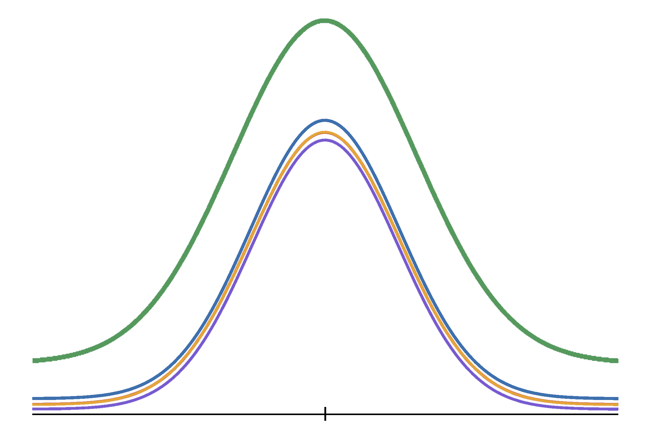
Use the interactive graph below to get a feel for how these two factors interact. The sliders for the means control the positions of the distributions, while the slider for the variability controls the shape of the distributions.

The #\green{\text{green line}}# indicates the position of the grand population mean.

The #\red{\text{red bar}}# indicates how strong the evidence against the null hypothesis is likely to be if we were to draw random samples from each of the populations.

ANOVA Logic Interactive