The notion of function

Functions: Functions

The notion of function

Functions

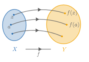
Let $\blue X$ and $\orange Y$ be sets.

A function $f$ of $\blue X$ to $\orange Y$ assigns one element of $\orange Y$ for each element $x$ from $\blue X$ . This element is denoted as ${f(x)}$ .

The notation $f : \blue X \to \orange Y$ indicates that $f$ is a function from $\blue X$ to $\orange Y$ .

We call $f(x)$ the value of the function (or short: value) of $f$ at $x$ . This is also called the image of argument $x$ under $f$ .

Machine

A function can be seen as a kind of machine. We put an element $x$ of $\blue X$ in the machine, and on the other side of the machine an element $f(x)$ of $\orange Y$ emerges. The machine calculates $f(x)$ according to rule determined by $f$ .

Example

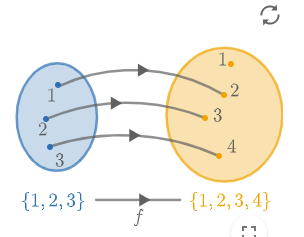
To the right is an example of $f: \blue{\{1,2,3\}} \to \orange{\{1,2,3,4\}}$ .

We can write the function $f$ as a line of numbers, namely $[2,3,4]$ .

This means:

$f(1)=2$

$f(2)=3$

$f(3)=4$

Relation

A function is in fact a special type of relation, as defined in sets. A function is actually a relationship between set $\blue X$ and $\orange Y$ . Here, an element $x$ of $\blue X$ relates to exactly one element of $\orange Y$ . This element is denoted by $f(x)$ .

Use of the letter f

We often denote a function using the letter $f$ , which comes from the word function. However, if we want to write a second function, we can not use the letter $f$ again, as it is already taken. We therefore often use the letter $g$ for the next function. When we want to write even more functions, we often just use the next letter in the alphabet.

It is also allowed to use, for example, letters from the Greek alphabet, such as $\alpha$ , $\phi$ or $\rho$ . We may even use multiple letters, e.g. an abbreviation.

In general, we like to keep the name of a function as short as possible. Therefore, we will write $T$ for temperature instead of $Temp$ or $Temperature$ .

Variable

Function rules can be given in the form $\orange y = f(\blue x)$ , where $f$ is the function and $\orange y$ is a variable abbreviating the function rule. We usually refer to $\orange y$ as the dependent variable, because it varies according to changes of $\blue x$ , and to $\blue x$ as the independent variable because we can choose $\blue x$ freely.

For instance, in the equation $\orange y=3\blue x +4$ , we can take $\blue x$ to be the independent variable so the equation defines a function $f(\blue x)$ with function rule $f(\blue x) = 3 \blue x +4$ .

The equation defines a relation between $\blue x$ and $\orange y$ that leads to a function. The use of dependent and independent variables makes it possible to switch the roles of $\blue x$ and $\orange y$ and obtain the inverse relation: we can take $\orange y$ to be the independent variable so as to obtain the function $g(\orange y)$ with function rule $g(\orange y) = \frac{1}{3}(\orange y - 4)$ . Now $\blue x$ is the dependent variable. In view of relations, the function $g$ represents the inverse relation to the one defined by $f$ .

We can represent functions in different ways. One of the most common ways is the function rule.

Function rule

A function rule for a function $f$ is an explicit expression to precisely show what the function does.

We write this as: $f(\blue x)=\ldots$ , where we enter an expression with a variable $\blue x$ replacing the dots. This algebraic expression tells us exactly what the function $f$ does.

The function rule cannot tell us which sets both $\blue x$ and $f(\blue x)$ have emerged from. Often, it is implicitly clear that $\blue x$ is a real number. We will talk more about this in the sections domain and range.

Examples

$\begin{array}{rcl}f(\blue x)&=&\blue x^2 \\ \\ g(\blue x)&=&\sqrt{\blue x} \\ \\ h(\blue x)&=&\blue x^3+\blue x+1 \end{array}$

Function value

Using the function rule, we can easily calculate the value of a function of an element.

Take the function on the right. If we want to calculate the value of the function at $\blue x=\blue2$ , we follow the function rule. Notice that we replace every $\blue x$ we encounter with $\blue2$ . We call this substitution.

The function value of $\blue x=\blue2$ therefore equals $4$ . We denote the value of $\blue x= \blue2$ with $f(\blue2)$ , i.e. $f(\blue2)=4$ .

In a similar way, we find that the value of $\blue x=\blue{-4}$ equals $16$ . In other words, $f(\blue{-4}) = 16$ .

Examples

$\begin{array}{rclcl} \text{From } f(\blue x)&=&\blue x^2 &\text{ then }&\\ \\f(\blue2)&=&\blue2^2&=&4 \\ \\&&\text{and}&& \\ \\f(\blue{-4})&=&\left(\blue{-4} \right)^2&=&16\end{array}$

Official notation

Above, we saw that we can describe a function using a function rule of the form $f(\blue x)=\ldots$ , in which whatever replaces the dots shows us what the function does.

Mathematicians often use the "maps to" arrow notation:

$f : \blue x \mapsto \ldots$

Here, too, whatever replaces the dots will tell us what the function does. The function value for an element $\blue x$ is still denoted with $f(\blue x)$ . In this way, a distinction is made between the function value and the function itself.

The reason that mathematicians use the "maps to" arrow notation is partly to clearly differentiate a function, an equation, and the function value. In practice, this difference is often clear from the context. In this course we will use the shorthand notation $f(\blue x)=\ldots$ .

In this course, we will use the notation $f : X \to Y$ , which is used to show us from which set to which set the function moves. The lowest examples on the right show what the official notation looks like when we also note the sets between which the function moves.

Examples

$\begin{array}{c}f :\blue x \mapsto \blue x^2 \\ \\ \\ g :\blue x \mapsto \sqrt{\blue x} \\ \\ \\ h : \blue x \mapsto \blue x^3+\blue x+1 \\ \\ \\ \\ f : \mathbb{R} \to \mathbb{R} , \blue x \mapsto \blue x^2 \\ \\ \\ g : \ivco{0}{\infty} \to \ivco{0}{\infty} ,\blue x \mapsto \sqrt{\blue x} \\ \\ \\ h : \mathbb{R} \to \mathbb{R} ,\blue x \mapsto \blue x^3+\blue x+1 \end{array}$

Piecewise defined function

It might seem that a function rule always looks like $f(\blue x) = \blue x^2$ , $f(\blue x) = 2\cdot \blue x +3$ , or anything similar. This is not always the case.

A function can also distinguish different situations. In that case, one expression applies for certain values of $\blue x$ , and another expression applies for other values of $\blue x$ .

In the examples, we can see the absolute value function, which for $\blue x \lt0$ is equal to $-\blue x$ and for $\blue x \geq 0$ equals $\blue x$ .
That means, for example, $f(\blue{-2})=2$ but $f(\blue3)=3$ .

This is also a function rule, because it tells us for each number $\blue x$ how the function value is calculated. We call a function by this form a piecewise defined function.

Examples

Absolute value function:

$f(\blue x)=\left\{\begin{array}{ll}-\blue x & \text{if } \blue x\lt0, \\ \blue x & \text{if } \blue x \geq 0.\end{array}\right.$

The absolute value function is often denoted as $f(\blue x)=|\blue x|$ .

Delta function:

$\delta_a(\blue x)=\left\{\begin{array}{ll}1 & \text{if } \blue x=a ,\\ 0 & \text{if } \blue x \ne a.\end{array}\right.$

Use of y

A function rule $f(\blue x) = \ldots$ is often denoted using $\orange y = \ldots$ . This means the same. The advantage is that this makes the function rule shorter. One drawback is that we can now make it more difficult to distinguish between two functions.

The two function rules $f(\blue x) = \blue x^2$ and $h(\blue x) = \blue x^3 +\blue x +1$ clearly denote two distinctly different functions. However, when we write this as $\orange y= \blue x^2$ and $\orange y = \blue x^3 + \blue x + 1$ , it seems like the $\orange y$ means two different things.

The use of the letters $\blue x$ and $\orange y$ is a habit. We might as well use $a$ and $b$ . Therefore, $\orange y = \blue x^2$ and $b = a^2$ often have the same meaning.

Examples

$\begin{array}{rcl}\orange y&=&\blue x^2 \\ \\ \\ \orange y&=&\sqrt{\blue x} \\ \\ \\ \orange y&=& \blue x^3+ \blue x+1 \end{array}$

Use of x

We often use the letter $\blue x$ in a function rule, but that is not mandatory. We may also use other letters. $\blue t$ is often used when we have a function denoting time, in which case the function rule becomes:

$f(\blue t)=\ldots$

Here, the dotted line will have an expression with $\blue t$ .

Examples

$\begin{array}{rcl}f(\blue t)&=&\blue t^2 \\ \\ g(\blue t)&=&\sqrt{\blue t} \\ \\ h(\blue t)&=& \blue t^3+ \blue t+1 \end{array}$

Consider the function:

$f(x)=\left(x+1\right)\cdot \left(x+6\right)$
Calculate the function value at $0$ .

The function value at $0$ is: $6$

To calculate the function value at $0$ , we substitute $x=0$ in the function.
We then get:

$f(0)=\left(0+1\right)\cdot \left(0+6\right)=6$
Hence, the function value at $0$ is $6$ .

New example