Random Variables

[A, SfS] Chapter 2: Probability: 2.4: Random Variables

Random Variables

In this lesson we learn about discrete and continuous random variables, their associated probability distributions, and computation of their means and variances

$\text{}$

Random Variable

Given an experiment with sample space $S$ consisting of all possible outcomes, a random variable associates a real number to each outcome in $S$ .

Although we call a r.v. a “variable”, it is actually a function, whose domain is $S$ and whose range is the subset of the real numbers to which the outcomes in $S$ are assigned by the function.

Notation

We usually denote a random variable (r.v.) with an upper-case letter from the latter part of the Latin alphabet, such as $X$ or $Y$ .

The range of r.v. $X$ is denoted $R(X)$ .

$\text{}$

Discrete Random Variable

If $R(X)$ is either finite or countable, then we say that $X$ is a discrete random variable.

Recall

A set of real numbers is countable if its elements can be placed in one-to-one correspondence with the positive integers. Otherwise, the set is uncountable.

For example, suppose an experiment involves flipping a coin $3$ times. In this case, the sample space is:

$S = \{HHH,HHT,HTH,THH,TTH,THT,HTT,TTT\}$

Let the r.v. $X$ be defined as the number of Heads in the $3$ coin flips. Then the range of $X$ is:

$R(X) = \{0,1,2,3\}$

Since $R(X)$ is finite, $X$ is a discrete r.v..

As you can see, each of the $8$ outcomes in $S$ is assigned by $X$ to one of the $4$ values in $R(X)$ .

As a second experiment, suppose an experiment involves counting the number of radioactive particles emitted by a specimen of uranium in one hour.

Then the sample space is:

$S=\{0,1,2,...\}$

Let the r.v. $Y$ be defined as the number of radioactive particles emitted by the specimen in one hour. Since $S$ is already a set of real numbers, it is convenient to define the range of $Y$ exactly the same way.

Thus the range of $Y$

$R(Y) = \{0,1,2,...\}$

is a countable set. So $Y$ is a discrete r.v..

$\text{}$

Continuous Random Variable

If the range of a r.v. $X$ is uncountable, we say that $X$ is a continuous random variable.

Suppose an experiment involved weighing (in grams) a specimen of rock taken from a geologic excavation site. Then the sample of this experiment is:

$S = (0,\infty)$

Let the r.v. $W$ be defined as the weight, in grams, of the rock. Since $S$ is already a set of real numbers, it is convenient to define the range of $W$ exactly the same way.

Thus the range of $W$

$R(W) = (0, \infty)$ is an uncountable set (an interval). So $W$ is a continuous r.v..

$\text{}$

Probability Distribution of a Discrete Random Variable

For a discrete r.v. $X$ , we define its probability distribution as the allocation of probability to each value in $R(X)$ .

Let $x$ denote one of the possible values for $X$ which is in the set $R(X)$ .

Then the probability of the event $X=x$ is the sum of the probabilities of all outcomes in $S$ which are assigned to the value of $x$ .

Probability Mass Function

The Probability Mass Function (pmf) of a discrete r.v. $X$ is a function $p(x)$ that gives us $\mathbb{P}(X = x)$ for each $x$ in $R(X)$ .

This function could be given in a table if $R(X)$ is not too large, or it could be given as a formula.

To be a legitimate pmf, it must be true that

$p(x) \geq 0$

for all $x$ in $R(X)$ and

$\sum_{x \ \text{in} \ R(X)}p(x) = 1$

Suppose an experiment involves flipping a coin $3$ times. The sample space of this experiment is:

$S = \{HHH,HHT,HTH,THH,TTH,THT,HTT,TTT\}$

Let the r.v. $X$ be defined as the number of Heads in the $3$ coin flips. Thus the range of $X$ is:

$R(X) = \{0,1,2,3\}$

The pmf of $X$ can be given in a table as:

$x$	$0$	$1$	$2$	$3$
$p(x)$	$\frac{1}{8} = 0.125$	$\frac{3}{8} = 0.375$	$\frac{3}{8} = 0.375$	$\frac{1}{8} = 0.125$

$\text{}$

The first row shows the values in $R(X)$ , and the second row shows the probability that $X = x$ for each $x$ in $R(X)$ , i.e., the probability mass function $p(x)$ .

As you can easily see, the sum of the four probabilities is $1$ .

As a second example, suppose an experiment involves counting the number of radioactive particles emitted by a specimen of Uranium in one hour.

Let the discrete r.v. $Y$ be defined as the number of radioactive particles emitted by the specimen in 1-hour. Thus the range of $Y$ is:

$R(Y) = \{0,1,2,...\}$

The pmf of $Y$ is given as a formula in this case:

$p(y) = e^{-0.9} \cdot \frac{0.9^y}{y!}$

for $y$ in $\{0,1,2,...\}$ .

It is not so obvious that the sum of $p(y)$ over all values in $R(Y)$ equals $1$ , but it is:

$\sum^{\infty}_{y=0} e^{-0.9} \cdot \frac{0.9^y}{y!} = e^{-0.9}\sum^{\infty}_{y = 0} \frac{0.9^y}{y!} = e^{-0.9} \cdot e^{0.9} = 1$

Here we used the Maclaurin series expansion for $e ^x$ which you learned in calculus:

$e^x = \sum^{\infty}_{n = 0}\frac{x^n}{n!}$

$\text{}$

Sometimes we are concerned not with the probability that a r.v. equals a specific value but with the probability that a r.v. is within a range of values.

Cumulative Distribution Function

For this, we define the cumulative distribution function $F(x) = \mathbb{P}(X \leq x)$ for each $x$ in the real numbers.

Based on this definition, $F$ is a non-decreasing function, i.e., if $x_1 > x_2$ then $F(x_1) \geq F(x_2)$ .

Since $F(x)$ is a probability, its value must be in the interval $[0,1]$ . Consequently, as $x \rightarrow - \infty$ , $F(x) \rightarrow 0$ , and as $x \rightarrow \infty$ , $F(x) \rightarrow 1$ .

Discrete Cumulative Distribution Function

For a discrete r.v. $X$ , its cdf is $F(x)= \sum_{t \leq x} p(t)$ .

Here we have the understanding that $p(t) = 0$ if $t$ is not in $R(X)$ . Consequently, the graph of $F$ will be a step function, with “jumps” at the real numbers which are in $R(X)$ .

For example, recall the experiment involving flipping a coin $3$ times, in which the r.v. $X$ was the same as the number of Heads in the $3$ coin flips.

The pmf of $X$ was given in a table as:

$x$	$0$	$1$	$2$	$3$
$p(x)$	$\frac{1}{8} = 0.125$	$\frac{3}{8} = 0.375$	$\frac{3}{8} = 0.375$	$\frac{1}{8} = 0.125$

$\text{}$

From this table we can see that for every $x < 0$ :

$F(x) = \mathbb{P}(X \leq x) = 0$

At $x = 0$ we accumulate a probability of $0.125$ , so for $0 \leq x < 1$ :

$F(x) = \mathbb{P}(X \leq x) = 0.125$

At $x = 1$ we accumulate an additional probability of $0.375$ to be added to the previous $0.125$ , so for $1 \leq x < 2$ :

$F(x) = \mathbb{P}(X \leq x) = 0.5$

At $x = 2$ we accumulate an additional probability of $0.375$ to be added to the previous $0.5$ , so for $2 \leq x < 3$ :

$F(x) = \mathbb{P}(X \leq x) = 0.875$

At $x = 3$ we accumulate an additional probability of $0.125$ to be added to the previous $0.875$ , after which no further probability can be accumulated, so for $3 \leq x < \infty$ :

$F(x) = \mathbb{P}(X \leq x) = 1$

We would write this as a piecewise-defined function:

$F(x) = \left\{\begin{array}{ll} 0 & \text{if} \ x < 0 \\ 0.125 & \text{if} \ 0 \leq x < 1 \\ 0.5 & \text{if} \ 1 \leq x < 2 \\ 0.875 & \text{if} \ 2 \leq x < 3 \\ 1 & \text{if} \ x \geq 3 \end{array} \right.$

The graph of $F(x)$ for this example looks like:

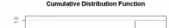
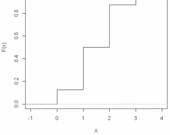
As you can see, as we go from left to right we are climbing up the steps from $0$ to $1$ , with the jumps occurring at each $x$ in $R(X)$ .

$\text{}$

Every random variable can be described with two parameters, its mean and its variance. We previously used these terms to describe the distribution of a quantitative variable on a population and on a sample. This is a different use of the terms, so you will need to keep the three uses sorted in your mind.

For a r.v., the mean signifies the center of the probability distribution, i.e., the value around which observations of the r.v. are centered.

The variance signifies how dispersed about the mean the observations of the r.v. tend be, i.e., whether the values are generally close to the mean or generally spread out around the mean.

Mean of a Discrete Random Variable

For a discrete r.v. $X$ with pmf $p(x)$ , the mean is denoted $\mu_X$ (or sometimes just $\mu$ if there is no danger of confusion), and is computed as:

$\mu_X = \sum_{x \ \text{in} \ R(X)}xp(x)$

The mean of $X$ is also known as the expected value of $X$ (or the expectation of $X$ ), in which case it is denoted as $E(X)$ .

Be sure you are comfortable with the equivalent terms and their notations, as we will use them interchangeably.

Variance and Standard Deviation of a Discrete Random Variable

The variance of a discrete r.v. $X$ with pmf $p(x)$ is denoted $\sigma^2_X$ (or, equivalently $V(X)$ ), and is computed as:

$\sigma^2_X = \sum_{x \ \text{in} \ R(X)}(x - \mu_X)^2p(x)$

With a little effort one can obtain an alternative form of this formula which is usually much easier to use:

$\sigma^2_X = \sum_{x \ \text{in} \ R(X)}x^2p(x) - \mu^2_X$

The standard deviation of a r.v. $X$ is simply the square root of the variance, and is denoted $\sigma_X$ .

If there is no danger of confusion, the variance and standard deviation can be denoted $\sigma^2$ and $\sigma$ respectively.

Recall again the experiment involving flipping a coin $3$ times, in which the r.v. $X$ was defined as the number of Heads in the $3$ coin flips.

The pmf of $X$ was given in a table as:

$x$	$0$	$1$	$2$	$3$
$p(x)$	$\frac{1}{8} = 0.125$	$\frac{3}{8} = 0.375$	$\frac{3}{8} = 0.375$	$\frac{1}{8} = 0.125$

$\text{}$

Hence the mean of $X$ is:

$\mu_X = (0)(0.125) + (1)(0.375) + (2)(0.375) + (3)(0.125) = 1.5$

And the variance of $X$ is:

$\sigma^2_X = (0)^2(0.125) + (1)^2(0.375) + (2)^2(0.375) + (3)^2(0.125) - 1.5^2 = 0.75$

Thus the standard deviation of $X$ is:

$\sigma_X = \sqrt{0.75} \approx 0.866$

Since the distribution of the number of Heads is symmetric from $0$ to $3$ it is not surprising that the center is at $1.5$ , which is halfway between $0$ and $3$ .

And since the middle $2$ values ( $1$ and $2$ ) are more probable than the extreme two values ( $0$ and $3$ ), the number of Heads deviates from $1.5$ by about $0.866$ , on average.

$\text{}$

Probability Density Function

If a random variable $X$ is continuous, it probability distribution is defined for all real numbers by a function $f(x)$ called its probability density function (pdf).

To be a legitimate pdf, we must have

$f(x) \geq 0$

for all $x$ , and

$\int^{\infty}_{-\infty}f(x)dx = 1$

Since the range of $X$ is in this case uncountable, it does not make sense to talk about $\mathbb{P}(X = x)$ . We can only compute probabilities for the r.v. to fall into an interval.

This is done by computing the area under the graph of its pdf above the interval, which usually involves integration. That is, for any two real numbers $a$ and $b$ with $a < b$ :

$\begin{array}{rcl} \mathbb{P}(a \leq X \leq b) &=& \int_a^b f(x)dx\\\\ \mathbb{P}(X \leq b) &=& \int_{-\infty}^b f(x)dx\\\\ \mathbb{P}(X \geq a) &=& \int_a^{\infty} f(x)dx \end{array}$

Important: For all three formulas above, the signs $\leq$ and $\geq$ can be replaced by $\lt$ and $\gt$ , since the area under the graph of $f(x)$ is not altered by exclusion of the endpoints. However, this is not true for discrete r.v.s! Be sure to keep this distinction clear in your mind.

$\text{}$

Cumulative Distribution Function

The cumulative distribution function (cdf) for a continuous r.v. $X$ is still defined as $F(x) = \mathbb{P}(X \leq x)$ , but now $F(x)$ is computed using integration.

That is, for every real number $x$ , $F(x) = \int_{-\infty}^x f(t)dt$ .

Note

We used a dummy variable $t$ inside the integral, since $x$ is being used as the upper limit.

In accordance with the Fundamental Theorem of Calculus, $F’(x) = f(x)$ at all continuity points of $f$ .

For example, the time (in seconds) until the next emission of a radioactive particles from a specimen, after the previous emission, can be modeled as the continuous r.v. $X$ with pdf $f(x) = 0.35 e^{-0.35x}$ for $x \geq 0$ , and $f(x) = 0$ for $x < 0$ .

The graph of the pdf is:

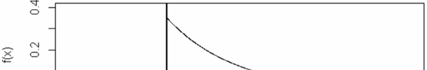
Clearly it is true that $f(x) \geq 0$ for all $x$ .

Also,

$\int_{-\infty}^{\infty}f(x)dx = \int_{0}^{\infty}0.35 e^{-0.35x}dx = \lim_{r\rightarrow \infty}\big[-e^{-0.35x}\big]_0^r = 1 - \lim_{r\rightarrow\infty}e^{-0.35r} = 1$

so $f(x)$ is a legitimate pdf.

What is the probability that the time until the next omission is more than $2$ seconds?

$\begin{array}{rcl} \mathbb{P}(X > 2) &=& \int_{2}^{\infty}0.35 e^{-0.35x}dx \\\\ &=& \lim_{r\rightarrow \infty}\big[-e^{-0.35x}\big]_2^r = e^{-0.7} - \lim_{r\rightarrow\infty}e^{-0.35r} = e^{-0.7} \approx 0.497 \end{array}$

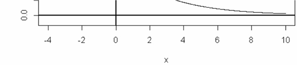
The cdf of $X$ is $F(x) = 0$ if $x < 0$ and $F(x) = \int_{0}^{x}0.35 e^{-0.35t}dt = 1 - e^{-0.35x}$ if $x \geq 0$ .

We write this cdf as a piecewise-defined function:

$F(x) = \left\{\begin{array}{ll} 0 & \text{if} \ x < 0 \\ 1 - e^{-0.35x} & \text{if} \ x \geq 0 \end{array} \right.$

The graph of the cdf is:

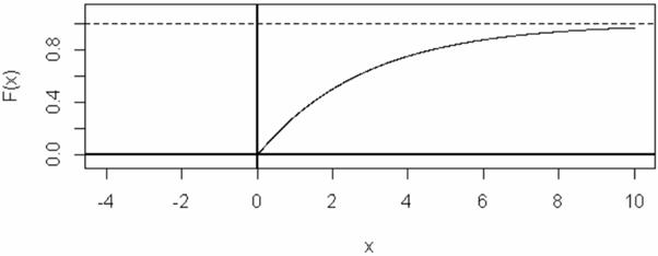
As you can see, the graph approaches $1$ as $x \rightarrow \infty$ , with a smooth curve on $(0, \infty)$ .

$\text{}$

Mean and Variance of a Continuous Random Variable

For a continuous r.v. $X$ with pdf $f(x)$ , the mean and variance of $X$ are computed as:

$\mu_X = \int_{-\infty}^{\infty}xf(x)dx$

and

$\sigma_X^2 = \int_{-\infty}^{\infty}(x - \mu_X)^2f(x)dx$

With some algebraic manipulation, the formula for the variance becomes:

$\sigma^2_X = \int_{-\infty}^{\infty} x^2f(x)dx - \mu_X^2$

which is generally much easier to compute.

As with discrete r.v.s, the mean of $X$ is also called the expectation of $X$ or the expected value of $X$ , denoted $E(X)$ , and the variance of $X$ can also be denoted $V(X)$ .

The standard deviation of $X$ is the square root of the variance, denoted $\sigma_X$ .

Again, the subscripts can be omitted if there is no danger of confusion.

For example, recall that the time (in seconds) until the next emission of a radioactive particle from a specimen, after the previous emission, can be modeled as the continuous r.v. $X$ with pdf:

$f(x) = 0.35e^{-0.35x}$

for $x \geq 0$ , and

$f(x) = 0$

for $x < 0$ .

What is the average time until the next omission? That would be the mean of $X$ , which is:

$\mu_X = \int_0^{\infty}0.35xe^{-0.35x}dx$

This requires the technique of integrating by parts, which results in $\mu_X = \frac{20}{7}$ . Note that the lower limit of the integral is $0$ rather than $-\infty$ , since $f(x) = 0$ for $x < 0$ .

The variance of $X$ is:

$\sigma^2_X = \int_0^{\infty}0.35x^2e^{-0.35x}dx - \big(\frac{20}{7}\big)^2$

which requires two iterations of integration by parts.

After a bit of effort, you get the result $\sigma_X^2 = \frac{400}{49}$ .

Then the standard deviation of $X$ is $\sigma_X = \frac{20}{7}$ , which is the same as the mean for this example.

$\text{}$

As with distributions of a variable on a population or on a sample, we can also refer to the quantiles of the probability distribution of a random variable. However, most of the quantiles will only make sense for a continuous r.v..

Quantiles of a Continuous Probability Distribution

For any number $q$ in (0,1), the $q$ th quantile of a continuous random variable $X$ with cdf $F(x)$ is the number $x_q$ that satisfies $F(x_q) = q$ .

If $p = 100q$ then $x_q$ can also be called the $p$ th percentile.

The median of $X$ is the $0.5$ quantile of $X$ , i.e., the $50$ th percentile of $X$ .

$\text{}$

We finish this section with an important result in probability that answers the question:

What is the probability that an observation of a r.v. falls more than $k$ standard deviations away from the mean?

The answer to this question depends on the probability distribution of the r.v., but we can derive an upper bound on this probability. This is given by Chebyshev’s Inequality.

Chebyshev’s Inequality

Chebyshev’s Inequality states that for any r.v. $X$ with mean $\mu_X$ and standard deviation $\sigma_X$ , the following property holds:

$\mathbb{P}\big(\big|X - \mu_X \big| \geq k\sigma_X \big) \leq \frac{1}{k^2}$

So, for example, the probability that an observation of a r.v. falls more than $2$ standard deviations away from its mean can be no larger than $\frac{1}{4}$ .

And the probability that an observation of a r.v. falls more than $3$ standard deviations away from its mean can be no larger than $\frac{1}{9}$ .