More Probability Distributions

[A, SfS] Chapter 3: Probability Distributions: 3.4: More Probability Distributions

More Probability Distributions

In this lesson, you will learn about three additional basic distributions encountered in statistics.

#\text{}#

There are three additional probability distributions, each continuous, that are encountered in this course.

Student's t-distribution

The first of these is the Student’s t-distribution with #\nu# degrees of freedom (#\nu# is the lower-case Greek letter “nu”). This distribution was developed by William Sealy Gosset, chief brewer for Guinness beer in Dublin, Ireland, in 1908. Because Guinness would not allow him to use his real name in his published work, he published it under the same name “the Student”.

The density curve for the t-distribution looks very much like that of a standard normal distribution, symmetric about #0# but with thicker tails and a lower peak. Its shape depends on the degrees of freedom. As #\nu# grows larger the density curve becomes indistinguishable from that of the standard normal density curve.

Student's t vs. Standard Normal Distribution

If a random variable #T# has the Student’s t-distribution with #\nu# degrees of freedom, we write #T \sim t_\nu#.

Also, the #p#th quantile of the #t_\nu# distribution is denoted #t_{\nu,p}#.

The value of #\nu# will depend on parameters that we will discuss later. We won’t show the formula for the pdf of this distribution here, but if you are curious you can find it online easily. Its mean is obviously #0# (as long as #\nu > 1#), and its variance is #\frac{\nu}{\nu - 2}# (as long as #\nu > 2#).

#\text{}#

Chi-Square Distribution

Another important distribution in statistics is the chi-square distribution with #k# degrees of freedom.

This distribution is the probability distribution of a sum of #k# squared standard normal random variables. Hence its range is #(0, \infty)#.

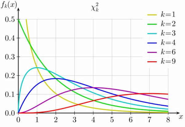
The shape of its density curve depends on #k#, as can be seen in this nice figure from Wikipedia:

The right side of the distribution is often called the “right tail”. There is of course no left tail.

If a random variable #X# has the chi-square distribution with #k# degrees of freedom, we write #X \sim \chi^2_k# (#\chi# is the lower-case Greek letter chi). Moreover, the #p#th quantile of the #\chi^2_k# distribution is denoted #\chi^2_{k,p}#.

The mean of a random variable having the #\chi^2_k# distribution is #k# and its variance is #2k#. The pdf can be found online if you are curious.

#\text{}#

F-Distribution

The last probability distribution that will be encountered in this course is the F-distribution with #d_1# and #d_2# degrees of freedom.

This is the probability distribution that results when one chi-square random variable (with #d_1# degrees of freedom) is divided by another chi-square random variable (with #d_2# degrees of freedom). Thus its range is also #(0, \infty)#.

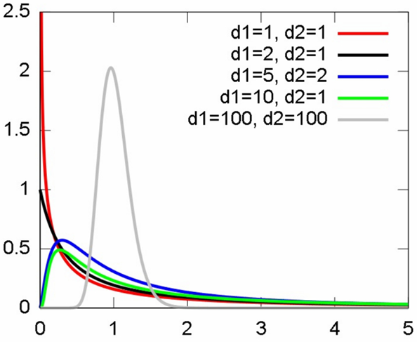
The shape of its density curve depends on the values of both #d_1# and #d_2#, as seen in this figure taken from Wikipedia:

This is a right-tailed distribution, like the chi-square distribution.

If a random variable #F# has the F-distribution with #d_1# and #d_2# degrees of freedom, we write #F \sim F_{d_1,d_2}#. Moreover, the #p#th quantile of this distribution is denoted #F_{d_1,d_2,p}#.

#\text{}#

Using R

Student's t-distribution

Suppose #T \sim t_\nu#.

Then to compute #P(T \leq t)# in #\mathrm{R}#, use:

> pt(t,v)

And to compute #P(T \geq t)# in #\mathrm{R}#, use:

> 1 - pt(t,v)

> pt(t,v,low=F)

#\text{}#

To compute the #p#th quantile of the #t_\nu#-distribution in #\mathrm{R}#, use:

> qt(p,v)

And to compute the #(1 - p)#th quantile use:

> qt(p,v,low=F)

#\text{}#

To generate a random sample of size #n# from the #t_\nu#-distribution in #\mathrm{R}#, use:

> rt(n,v)

Chi-square distribution

Next, suppose #X \sim \chi_k^2#.

Then to compute #P(X \leq x)# in #\mathrm{R}#, use:

> pchisq(x,k)

And to compute #P(X \geq x)# in #\mathrm{R}#, use:

> 1 - pchisq(x,k)

> pchisq(x,k,low=F)

#\text{}#

To compute the #p#th quantile of the #\chi_k^2#-distribution in #\mathrm{R}#, use:

> qchisq(p,k)

And to compute the #(1 - p)#th quantile use:

> qchisq(p,k,low=F)

#\text{}#

To generate a random sample of size #n# from the #\chi_k^2#-distribution in #\mathrm{R}#, use:

> rchisq(n,k)

F-distribution

Now suppose #F \sim F_{d_1,d_2}#.

Then to compute #P(F \leq f)# in #\mathrm{R}#, use:

> pf(f,d1,d2)

And to compute #P(F \geq f)# in #\mathrm{R}#, use:

> 1 - pf(f,d1,d2)

> pf(f,d1,d2,low=F)

#\text{}#

To compute the #p#th quantile of the #F_{d_1,d_2}#-distribution in #\mathrm{R}#, use:

> qf(p,d1,d2)

And to compute the #(1 - p)#th quantile use:

> qf(p,d1,d2,low=F)

#\text{}#

To generate a random sample of size #n# from the #F_{d_1,d_2}#-distribution in #\mathrm{R}#, use:

> rf(n,d1,d2)