[A, SfS] Chapter 7: Chi-square tests and ANOVA: 7.3: One-way Analysis of Variance
 One-way Analysis of Variance
One-way Analysis of VarianceIn this section, we will discuss how can we assess whether the population means of a continuous variable are different for different groups.
Consider a setting in which we have a continuous variable #Y#, which we call the response or outcome variable, whose values may depend on the levels of one or more categorical variables, which we call factors.
In the sciences, this setting often arises in a factorial experiment, in which subjects (the experimental units) are assigned to treatment groups which are distinguished by various combinations of treatments. All members of the same treatment group are called replicates.
In a completely randomized experiment, the experimental units are assigned to the treatments at random, with an equal likelihood of being assigned to each group. If the combinations of treatments experienced by each group are pre-determined by the experimenter, the experimental results can be analyzed using a fixed-effects model. But if the combinations of treatments occur randomly, a much more complicated random-effects model is necessary. In this course, we will only study fixed effects.
\[\text{}\]
One-factor ExperimentIn a one-factor experiment, the treatment groups are distinguished by the level of a single categorical factor.
For example, consider an experiment in which the response variable is the change in systolic blood pressure, and the factor is the type of video clip viewed.
Suppose there are five levels (categories) for this factor: the baseline level, which views a neutral video clip, and four other levels corresponding to different video clips showing one of four different intense action scenes: a car chase, a sword fight, skiing down an expert-level slope, and a boxing match.
The research question is whether the type of video clip watched has some influence on the blood pressure within some specified population. In other words, is the mean change in systolic blood pressure the same no matter which video clip is viewed?
In general, the factor has #I# levels, and the population mean for the response variable #Y# for level #i# is #\mu_i#, for #i = 1,...,I#. Meanwhile, #\mu# is the overall mean of the response variable #Y# for the population across all levels of the factor.
One-Way ANOVA Model and HypothesesThe one-way Analysis of Variance model for the value of the response variable #Y# for a subject randomly-selected from level #i# of the factor is:\[Y_i = \mu_i + \varepsilon\]
where #\varepsilon# is a random variable with mean #0# and some unknown variance #\sigma^2#. We usually further specify that #\varepsilon# is normally-distributed on the population.
We call #\varepsilon# the error, by which we mean the amount by which the value of #Y# deviates from #\mu_i# for a randomly-selected subject from group #i#.
In this context, we wish to test the following hypotheses:
\[\begin{array}{rl}
H_0:&\mu_1 = \cdots = \mu_I \text{ (the mean of the response is the same for all levels of the factor, i.e., the factor has}\\
&\text{no significant effect on the response)}\\\\
H_1 :& \mu_i \neq \mu_j \text{ for at least one pair of levels }(i,j) \text{ (the mean of the response is not the same for at least}\\
&\text{one pair of levels of the factor, i.e., the factor has some significant effect on the response)}
\end{array}\]
Note: usually #I > 2#, otherwise this is just a test for difference in means.
\[\text{}\] Assume that we have #N# subjects involved in the experiment, with #n_i# subjects assigned to level #i#, for #i = 1,...,I#. Thus \[N = n_1 + \cdots + n_I\] If #n_i# is the same for each #i#, the experiment has a balanced design, which makes the hypothesis test less sensitive to departures from the assumptions (to be introduced shortly).
Sample Mean and Grand Sample MeanLet #Y_{ij}# denote the measured value of the response for the #j#th replicate in the treatment group corresponding to level #i# of the factor.
Let \[\bar{Y}_i = \cfrac{1}{n_i}\sum^{n_i}_{j=1}Y_{ij}\] denote the sample mean for the treatment group corresponding to level #i#, which is an unbiased estimate of #\mu_i#.
Let \[\bar{Y} = \cfrac{1}{N}\sum^I_{i=1}\sum^{n_i}_{j=1}Y_{ij} = \cfrac{1}{N}\sum^I_{i=1}n_i\bar{Y}_i\] denote the sample grand mean across all treatment groups, which is an estimate of the population grand mean #\mu#.
Thus if #H_0# is true, each #\bar{Y}_i# should be close to #\bar{Y}#, relative to the sample variability within the individual treatment groups.
Consequently, we compare the variance between the groups to the variance within the groups, which is why the procedure is called the Analysis of Variance (ANOVA). When there is only one factor involved, it is called One-Way ANOVA.
\[\text{}\] To conduct inference, several assumptions must be satisfied.
One-way ANOVA AssumptionsLet \[Y_{ij} = \mu_i + \varepsilon_{ij}\] denote the value of the response variable for the #j#th replicate randomly-assigned to treatment group #i# from the population. Thus #Y_{ij}# has mean #\mu_i# and randomly deviates from this mean by #\varepsilon_{ij}#.
As stated previously, we assume that the error \[\varepsilon_{ij} \sim N\Big(0,\sigma^2\Big)\] in this model, where #\sigma^2 > 0# does not depend on #i#.
This is the same as assuming: \[Y_{ij} \sim N\Big(\mu_i,\sigma^2 \Big)\] Consequently, for #i = 1,...,I#, the variance of #\bar{Y}_i# is #\cfrac{\sigma^2}{n_i}#.
The assumption that #\sigma^2# is the same for all the treatment groups is called constant variance or homoscedasticity.
This assumption can be checked by checking the residuals #Y_{ij} - \bar{Y}_i# for #i = 1,...,I# and #j = 1,...,n_i# for each #i#. This is because the residuals should represent a random sample from the #N\Big(0,\sigma^2\Big)# if the assumptions are true.
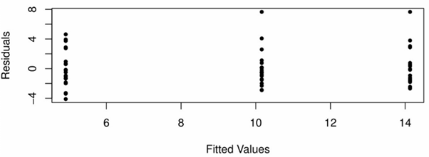
A scatterplot of these residuals against the corresponding fitted values #\bar{Y}_1,...\bar{Y}_I# should show approximately the same spread for each fitted value, and no extreme outliers, as seen in the following plot:

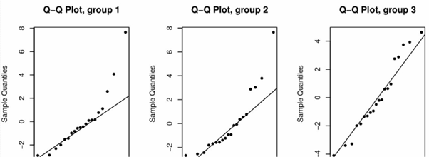
Furthermore, for each #i# a Normal quantile-quantile plot should also be used to confirm the assumption of normality of #Y_{ij}# for each level #i#. The following plot casts doubt on this assumption for group 1 and group 2:


Using the above plots to assess the validity of these two assumptions is a qualitative approach. We can formally assess the validity of the two assumptions using various hypothesis tests. The Shapiro-Wilk test is a commonly-used test for the normality assumption, while Bartlett's test is commonly used to test the constant variance assumption. For both tests we do not want to reject the null hypothesis.
\[\text{}\] The test statistic of an ANOVA is calculated on the basis of two types of variance: the between-groups variance and the within-groups variance.
One-way ANOVA Test Statistic and Null DistributionLet \[SSTr = \sum^I_{i=1}n_i\Big(\bar{Y}_i - \bar{Y}\Big)^2\] denote the treatment sum of squares.
Then let \[MSTr = \cfrac{SSTr}{I - 1}\] denote the treatment mean square. This is a measure of the variance of the treatment group sample means around the sample grand mean, i.e., the between-groups variance.
Next, let \[SSE = \sum^I_{i=1}\sum^{n_i}_{j=1}\Big(Y_{ij} - \bar{Y}_i\Big)^2\] denote the error sum of squares.
Finally, let \[MSE = \cfrac{SSE}{N - I}\] denote the mean square error. This is a measure of the variance of the replicates in each treatment group around their treatment group sample mean, i.e., the within-groups variance, and thus is an unbiased estimate of #\sigma^2#.
If the assumptions are satisfied, the statistic \[F = \cfrac{MSTr}{MSE}\] has the #F_{I - 1,N-I}# distribution.
The P-value of the test is computed as #P(F \geq f)#, where #f# is the observed value of #F#. Statistical software typically displays this information in an ANOVA table.
A small P-value is evidence against #H_0# and supports the conclusion that the population means #\mu_1,...,\mu_I# are not the same for all treatment groups, i.e., that the factor has a significant effect on the response.
\[\text{}\]We might like to compute #(1 - \alpha)100\%# confidence intervals for #\mu_i# for each level #i#.
One-Way ANOVA Confidence IntervalWhen conducting an ANOVA, each population group mean #\mu_i# is estimated by #\bar{Y}_i#, and the variance of #\bar{Y}_i# is estimated by #\cfrac{MSE}{n_i}#.
Then, when the assumptions are satisfied, it is true that: \[\cfrac{\bar{Y}_i - \mu_i}{\sqrt{MSE/n_i}} \sim t_{N-I}\] So for any #\alpha# in #(0,1)#, a #(1 - \alpha)100\%# confidence interval for #\mu_i# is: \[\bigg(\bar{Y}_i - t_{N-I,\alpha/2}\sqrt{\cfrac{MSE}{n_i}},\,\,\, \bar{Y}_i + t_{N-I,\alpha/2}\sqrt{\cfrac{MSE}{n_i}}\bigg)\]
\[\text{}\]
One-Way ANOVA in R#\mathrm{R}# can be used to efficiently conduct analysis of variance (ANOVA). We demonstrate this using the following data, which you can copy and paste into #\mathrm{R}#:
> Y = c(24.6,22.8,27.5,21.3,24.0,33.4,25.2,19.6,29.4,20.8,32.7,23.3,18.2,28.7,24.0)

> Group = c(2,1,3,1,2,3,2,1,3,1,3,2,1,3,2)

> Data = data.frame(Y, Group)
Here #\mathtt{Y}# is the response variable, and #\mathtt{Group}# is the categorical factor, which has 3 levels.
There are #15# subjects, and the #k#th position in the two vectors gives the group level and the response variable measurement for the #k#th subject, for #k = 1,...,15#. We merge these together into a data frame which we aptly name #\mathtt{Data}#. (If you read data into #\mathrm{R}# from a file using the #\mathtt{read.table()}# function, it will be loaded as a data frame. You can give it any name you like, though Data usually makes the most sense.)
We have a one-factor experiment, with #\mathtt{Y}# as the response variable and #\mathtt{Group}# as the factor. We can create a model in #\mathrm{R}# using the #\mathtt{aov()}# function and then inspect the results using the #\mathtt{summary()}# function as follows:
> Model = aov(Y ~ factor(Group), data=Data)

> summary(Model)
We stored the output from the #\mathtt{aov()}# function in an object that we named #\mathtt{Model}#. You can choose any name you like.
Note that we have to convert the numeric vector #\mathtt{“Group”}# into the factor class in #\mathrm{R}# using the #\mathtt{factor()}# function if we want the #\mathtt{aov() }# function to work properly. Even if #\mathtt{Group}# was already in the factor class, using the #\mathtt{factor()}# function would do no harm, so to be on the safe side it is a good idea to always do this.
Note also that the #\mathtt{aov()}# function allows us to specify the data frame in which to find the variables, so that we don't have to type #\mathtt{Data$Y}# and #\mathtt{Data$Group}#. If the variables are not nested inside a data frame, but are in the #\mathrm{R}# workspace, then we would not use the #\mathtt{“data=”}# setting.
The output of the #\mathtt{summary()}# function is an ANOVA table (which we can also obtain using #\mathtt{anova(Model)}#), which allows us to see the treatment sum of squares (in the first row, after #\mathtt{“factor(Group)”}#) and the error sum of squares (in the second row, after #\mathtt{“Residuals”}#), preceded by their respective degrees of freedom and followed by their mean squares, the F-statistic and the P-value for the F-test of the null hypothesis #H_0: \mu_1 = \mu_2 = \mu_3# against the alternative hypothesis #H_1: \mu_i \neq \mu_j# for at least one pair #i# and #j#:
| Df | Sum Sq | Mean Sq | F value | Pr(>F) | |
| factor(Group) | 2 | 245.06 | 122.53 | 36.1 | 8.38e-06*** |
| Residuals | 12 | 40.73 | 3.39 |
Signif.codes: 0'***' 0.001'**' 0.01'*' 0.05'.' 0.1'' 1
The #\mathtt{“Signif.codes”}# let you know how small the P-value of the F-test is, in case you can't figure that out yourself.
Here the given P-value translates as #0.00000838#, which is between #0# and #0.001#, as signified by #3# stars. So we would reject the null hypothesis and conclude that there are at least two population means which differ out of the three groups. However, this conclusion is only valid if the assumptions are satisfied.
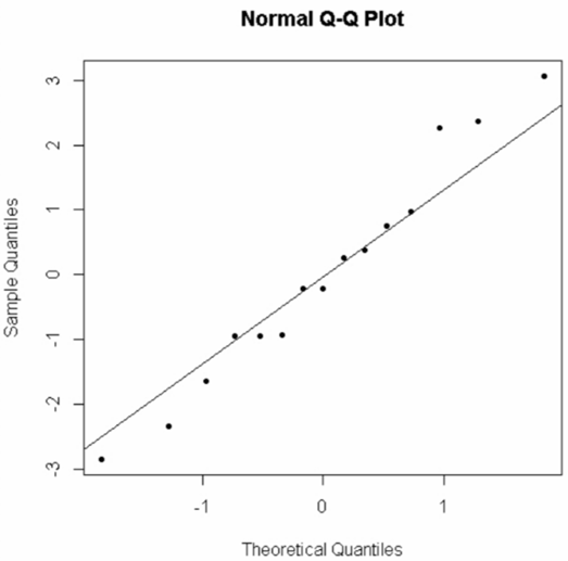
To qualitatively check the normality of #\mathtt{Y}# in each group, we can use a single Q-Q-plot of the model residuals:
> qqnorm(Model$residuals, pch=20)

> qqline(Model$residuals)
We get:

The points are close enough to the line that we would not reject the assumption of normality.
There is also a hypothesis test, called the Shapiro-Wilk test, available in #\mathtt{R}#, whereby you can formally test #H_0#: the residuals come from a normal distribution, against #H_1#: the residuals do not come from a normal distribution. In #\mathtt{R}#, use:
> shapiro.test(Model$residuals)
A small P-value implies that the residuals do not come from a normal distribution, which in turn implies that the dependent variable is not normally-distributed in each group of the factor. This violates the assumption and makes any inference based on that assumption invalid.
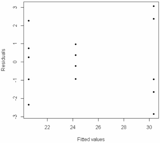
To qualitatively check the assumption of constant variance (homoscedasticity), we can make a scatterplot of the model residuals against the fitted values (i.e., the group sample means):
> plot(Model$fitted.values, Model$residuals, pch=20, xlab="Fitted values", ylab="Residuals")

The spread of points in the middle group (group 2) is smaller than the spread of points in the other two groups, which indicates we may have a problem with the constant variance assumption. But this is hard to address visually.
There is also a hypothesis test, called Barlett's test, available in #\mathtt{R}#, whereby you can formally test #H_0#: the variance is the same in all groups of the factor, against #H_1#: the variance is not the same in all groups of the factor. In #\mathtt{R}#, this test can be performed for the above data as follows:
> bartlett.test(Y~factor(Group), data=Data)
A small P-value implies that the constant variance assumption is violated, and thereby invalidates any inference based on this assumption.
For the data, if you need the group sample means, along with the overall mean (the "grand mean"), use the #\mathtt{model.tables()}# function, with the setting #\mathtt{type=“means”}#:
> model.tables(Model, type="means")
However, if you want confidence intervals for the population means, you have to first fit a new model with a small adjustment: you have to put '#\mathtt{0 +}#' after the '#\mathtt{\sim}#' symbol.
Then you can use the #\mathtt{confint()}# function on this adjusted model to obtain confidence intervals for the population means in each group, at any specified confidence level (default is 95%):
> Model2 = aov(Y ~ 0 + factor(Group), data=Data)

> confint(Model2, level=0.99)
We get the output:
| 0.5% | 99.5% | |
| factor(Group)1 | 18.02326 | 23.05674 |
| factor(Group)2 | 21.70326 | 26.73674 |
| factor(Group)3 | 27.82326 | 32.85674 |
We can see that the #99\%# CI for the mean of group 3 has no overlap with the #99\%# CIs for the means of the other two groups, so it seems very clear that group 3 has a larger mean than groups 1 and 2.
Example:
Archaeologists can determine the diets of ancient civilizations by measuring the ratio of carbon-13 to carbon-12 in bones found at burial sites. Large amount of carbon-13 suggests a diet rich in grasses such as maize, while small amounts suggest a diet based on herbaceous plants.
An article from 2002 reports ratios, as a difference from a standard in units of parts per thousand, for bones from individuals in several age groups. The data can be pasted into #\mathrm{R}# using the below code:
> Data = data.frame(Ratio=c(17.2,18.4,17.9,16.6,19.0,18.3,13.6,13.5,18.5,19.1,19.1,
13.4,14.8,17.6,18.3,17.2,10.0,11.3,10.2,17.0,18.9,19.2,18.4,13.0,14.8,18.4,12.8,17.6,
18.8,17.9,18.5,17.5,18.3,15.2,10.8,19.8,17.3,19.2,15.4,13.2,15.5,18.2,12.7,15.1,18.2,
18.0,14.4,10.2,16.7), Age.Group=c(rep(1,12),rep(2,10),rep(3,18),rep(4,9)))
Here age group 1 is ages #0# to #11# years, age group 2 is ages #12# to #24# years, age group 3 is #25# to #45# years, and age group 4 is ages #46# years and older.
Test the null hypothesis that the population mean ratio does not differ among the four age groups against the research hypothesis that the population mean ratio is different among the four age groups.
Produce the ANOVA table, including the P-value of this test, and state the appropriate conclusion. Also report #95\%# CIs for the population mean ratio of each age group.
Solution:
In #\mathrm{R}# we do as follows:
> Model = aov(Ratio ~ factor(Age.Group), data=Data)

> summary(Model)
The output gives the ANOVA table:
| Df | Sum Sq | Mean Sq | F value | Pr(>F) | |
| factor(Age.Group) | 3 | 21.0 | 6.988 | 0.891 | 0.453 |
| Residuals | 45 | 352.9 | 7.843 |
Based on the large P-value of #0.453#, we do not reject the null hypothesis. So we cannot conclude that the ratios differ among the age groups.
We can obtain #95\%# CIs for the population mean ratio for each of the 4 groups as follows:
> Model2 = aov(Ratio ~ 0 + factor(Age.Group), data=Data)

> round(confint(Model2), 2)
This gives us:
| 2.5% | 97.5% | |
| factor(Age.Group)1 | 15.42 | 18.68 |
| factor(Age.Group)2 | 13.67 | 17.23 |
| factor(Age.Group)3 | 15.16 | 17.82 |
| factor(Age.Group)4 | 13.56 | 17.32 |
We can see that all four CIs overlap substantially, which is consistent with our findings above.

Or visit omptest.org if jou are taking an OMPT exam.


