Simple Linear Regression

[A, SfS] Chapter 8: Correlation and Regression: 8.2: Simple Linear Regression

Simple Linear Regression

Simple Linear RegressionIn this section, we will discuss how we can model the linear relationship between a continuous dependent variable and a quantitative independent variable using a linear function.

In many scientific studies, we have a continuous variable $Y$ which we hypothesize to have an association with some other quantitative variable $x$ . This hypothesis could be based on theory, such as a physical law, or based on observations, in which case we develop an empirical model, i.e., a model which seems to be useful but which does not necessarily reflect some underlying objective truth. In this kind of model, we are thinking in terms of explaining the variation in $Y$ using the variable $x$ , which could allow us to make predictions for the value of $Y$ when the value of $x$ is given.

If we believe that the association between two quantitative variables is linear, then we employ a linear model to represent that association, i.e., an equation

$Y = \beta_0 + \beta_1x$ for some real constants $\beta_0$ and $\beta_1$ representing the $Y$ -intercept and slope of a line, respectively.

However, when looking at data it is evident that observed values of $Y$ for different values of $x$ do not precisely conform to such a linear function, no matter what values are chosen for $\beta_0$ and $\beta_1$ . The $Y$ values deviate from the model, either in the positive or the negative direction, with some of these deviations much larger than others.

To incorporate this behavior into our linear model, we must include an error term $\varepsilon$ , which we treat has a random variable with mean $0$ and some variance $\sigma^2$ that accounts for the variability of the observations around the linear function. Thus the linear model becomes:

$Y = \beta_0 + \beta_1x + \varepsilon$ In this model, we call $Y$ the dependent variable (DV), or alternatively, the response variable or the outcome variable. We call $x$ the independent variable (IV), or alternatively, the explanatory variable or the predictor or the covariate.

The IV $x$ is not a random variable, but since $\varepsilon$ is a random variable, the DV $Y$ is also random, with its mean dependent on $x$ , i.e.,

$E(Y|x) = \beta_0 + \beta_1x$ and variance $\sigma^2$ .

The values of the coefficients $\beta_0$ and $\beta_1$ are based on the proposed linear association at the population level and are usually not known (unless derived from theory, as in a physics equation). Consequently, we must estimate the values using a random sample from the population. We will denote the estimates by $\hat{\beta}_0$ and $\hat{\beta}_1$ , respectively.

The process of using data to obtain the estimates $\hat{\beta}_0$ and $\hat{\beta}_1$ is called linear regression.

When there is only one independent variable, the process is called simple linear regression.

There are different procedures for obtaining the estimates, including the method of maximum likelihood. But we will use a method called ordinary least-squares regression (OLS), in which case $\hat{\beta}_0$ and $\hat{\beta}_1$ are called the least-squares coefficients, and the resulting linear equation

$y = \hat{\beta}_0 + \hat{\beta}_1x$ is called the equation of the least-squares regression line.

This is understood to be the equation of the best-fit line which fits the points in the scatterplot better than any other line. Of course, "best fit" implies that there must be some criterion by which we decide what is indeed the best fit. That criterion is the least-squares criterion.

Least-squares CriterionGiven measurements of the variables $x$ and $y$ on a random sample of size $n$ from the population, we obtain observed pairs $(x_1,y_1),...,(x_n,y_n)$ .

Suppose for a moment that we already have the estimates $\hat{\beta}_0$ and $\hat{\beta}_1$ . Then given any arbitrary observed pair $(x_i,y_i)$ , we can use $x_i$ in the equation of the regression line to obtain the predicted value of $y_i$ (also called the fitted value) $\hat{y}_i$ , i.e.,

$\hat{y}_i = \hat{\beta}_0 + \hat{\beta}_1x_i$

This is the value that the estimated linear model predicts for the DV $y$ when $x = x_i$ . The predicted value is almost always different from the observed value $y_i$ , so let

$e_i = y_i - \hat{y}_i$ denote the residual corresponding to $(x_i,y_i)$ .

The best-fit model would make $e_i$ as small as possible. But because there are $n$ pairs $(x_i,y_i)$ , and they do not all lie precisely on the same line, it will not be possible to make all the residuals equal to zero. Instead, we want to make them collectively as small as possible.

In the method of least-squares, we minimize the sum of the squared residuals, which we denote as

$\begin{array}{rcl} S &=& \displaystyle\sum_{i=1}^n e^2_i \\\\ &=& \displaystyle\sum_{i=1}^n \Big(y_i - \hat{y}_i \Big)^2 \\\\ &=& \displaystyle\sum_{i=1}^n\Big(y_i - \hat{\beta}_0-\hat{\beta}_1x_i\Big)^2 \end{array}$

Our goal is to choose $\hat{\beta}_0$ and $\hat{\beta}_1$ such that we minimize $S$ .

To accomplish this, we find the derivative of $S$ with respect to each coefficient separately, set each derivative equal to $0$ , and solve the two resulting equations simultaneously to obtain these values. We also check the second derivatives to be sure we have found a minimum.

In the end, we find the least-squares coefficients to be given by the formulas:

$\begin{array}{rcl} \hat{\beta}_1 &=& \cfrac{\displaystyle\sum_{i=1}^n(x_i - \bar{x})(y_i - \bar{y})}{\displaystyle\sum_{i=1}^n(x_i - \bar{x})^2} \\\\ &=& \cfrac{\displaystyle\sum_{i=1}^n x_iy_i - n\bar{x}\bar{y}}{\displaystyle\sum_{i=1}^nx_i^2 - n\bar{x}^2}\end{array}$ and

$\hat{\beta}_0 = \bar{y} - \hat{\beta}_1 \bar{x}$

Note that one can also compute the slope estimate using the Pearson sample correlation coefficient $r$ , i.e., the slope of the least-squares regression line is:

$\hat{\beta}_1 = r \cdot \cfrac{s_y}{s_x}$ The least-squares regression line always passes through the point $(\bar{x},\bar{y})$ , and its slope is the estimated average change in the value of the DV for each one-unit increase in the value of the IV.

In the following plot, the data were simulated from the linear model

$Y = -1 + 5x + \varepsilon$ with $\varepsilon \sim N(0,625)$ .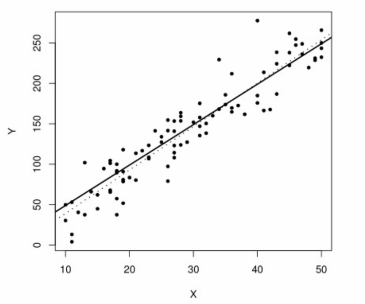

The least-squares coefficients are computed as $\hat{\beta}_0 = -14.41$ and $\hat{\beta}_1 = 5.37$ . Although the intercept estimate is quite inaccurate, the slope estimate is very close to the truth.

Both the true line (solid) and the regression line (dotted) are plotted together with the data. As can be seen, the regression line is not far from the true line, and fits the scatterplot quite well.

The line

$y = \hat{\beta}_0$ + $\hat{\beta}_1x$

is the best-fit line to model the association implicit within the given data, and is an unbiased estimate of the hypothetical line

$y = \beta_0 + \beta_1x$ that describes the association between the two variables $x$ and $y$ at the population level.

However, it only describes that association for the range of observed values for the IV (in the above example, from $10$ to $50$ ). It is unwise to extrapolate this model to values of the IV outside of that range. In the above example, if we extrapolate the model to values of $x$ close to $0$ , we already know that the model will be very inaccurate, since the true intercept and the estimated intercept are very different.

Although the model is the best linear fit for the data, it does not mean that the fit is particularly good. It just means that no other line fits the data better, based on the least-squares criterion.

$\text{}$ We would like to have a measure of the quality of the fit of the model to the data.

Determining the Quality of the Model's FitLet $SST$ denote the total sum of squares for the DV, defined as:

$SST = \displaystyle\sum_{i=1}^n(y_i - \bar{y})^2$ This represents the total variability in our sample of the DV around its mean value, without considering the association with the IV.

Meanwhile, the sum of the squared residuals (given above as $S$ ) is also known as the error sum of squares $SSE$ , and represents the total variability in our sample of the DV around the regression line.

$SSE = S = \displaystyle\sum_{i=1}^n \Big(y_i - \hat{y}_i \Big)^2$ If the model fits well, the $SSE$ should be small relative to the $SST$ .

Let $SSR$ denote the regression sum of squares, defined as:

$SSR = SST - SSE$ So if $SSE$ is small relative to $SST$ , then $SSR$ would be large relative to $SST$ .

To measure the goodness of the fit of the model to the data, we define the coefficient of determination $R^2$ as:

$R^2 = \cfrac{SSR}{SST} = 1 - \cfrac{SSE}{SST}$ Thus $R^2$ may be interpreted as the proportion of the total variance in the DV which can be explained by its linear association with the IV. This choice of notation is not coincidental, because in the simple linear model the coefficient of determination is the same as the square of the Pearson correlation coefficient $r$ between the observed values of the DV and the IV.

Consequently, $R^2$ is always between $0$ and $1$ , and the closer $R^2$ is to $1$ the better is the quality of the fit of the linear model to the data, and the better is the usefulness of the model to predict the value of the DV for given values of the IV.

Note that there is no established threshold for distinguishing a "good fit" from a "bad fit". But if we compare two or more simple linear models for the DV, we can use this criterion to conclude which model has the best fit among them.

For the model derived from the previous figure, we have $R^2 = 0.8838$ , so we can say that the linear model explains $88.38\%$ of the variability in the DV, which is quite good.

$\text{}$ Now for some statistical inference about the population parameters for the linear model.

Inference about the Parameters of a Simple Linear ModelWe have assumed that the error $\varepsilon$ in the model

$Y = \beta_0 + \beta_1x + \varepsilon$ is a random variable with mean $0$ and variance $\sigma^2$ .

We now assume further that $\varepsilon \sim N\Big(0,\sigma^2\Big)$ .

Consequently, for any specified value of $x$ , it is true that:

$Y | x \sim N \Big(\beta_0 + \beta_1x,\sigma^2\Big)$ Based upon these assumptions, we can derive the following:

An unbiased estimate of the error variance $\sigma^2$ is the mean-square error: $MSE = \cfrac{SSE}{n - 2}$ Since $R^2 = 1 - \cfrac{SSE}{SST}$ we have $SSE = (1 - R^2) SST$ so an alternative formula is: $MSE = \cfrac{(1 - R^2)SST}{n - 2}$
The variance of $\hat{\beta}_1$ , denoted $\sigma^2_1$ , is estimated by $s^2_1 = \cfrac{MSE}{(n - 1)s^2_x}$ where $s_x^2 = \cfrac{1}{n-1}\displaystyle\sum_{i-1}^n(x_i - \bar{x})^2$ .

Its square root $s_1$ is the standard error of the slope estimate.
The variance of $\hat{\beta}_0$ , denoted $\sigma^2_0$ , is estimated by $s^2_0 = MSE \bigg(\cfrac{1}{n} + \cfrac{\bar{x}^2}{(n-1)s_x^2}\bigg)$ Its square root $s_0$ is the standard error of the intercept estimate.

The statistics $T_0 = \cfrac{\hat{\beta}_0 - \beta_0}{s_0} \,\,\,\,\,\,\text{and}\,\,\,\,\,\, T_1 = \cfrac{\hat{\beta}_1 - \beta_1}{s_1}$ each have the $t_{n-2}$ distribution.

Thus we can compute confidence intervals for $\beta_0$ and $\beta_1$ , or conduct hypothesis tests regarding the values of $\beta_0$ and $\beta_1$ , using the same formulations that we used when we made inference about the population mean $\mu$ of a quantitative variable using the Student's t-distribution. The null hypothesis value for the slope would be denoted $\beta_{10}$ and for the intercept would be denoted $\beta_{00}$ .

Typically we are interested in testing whether the slope $\beta_1$ of the regression line is different from zero. A nonzero slope implies that the IV has a statistically significant effect on the DV. Most statistical software will report the P-value for this particular test (along with a test for the value of the intercept, which is rarely of interest).

Another topic of statistical inference is estimating the population mean of the DV for any specified value of the IV, i.e., $E(Y|x)$ . We skip that in this course.

Also, we might want to use the linear model to predict the value of the DV for a single future observation having a specified value of the IV, using a prediction interval. We will also skip this topic in this course.

$\text{}$

Using RSimple Linear Regression

To conduct simple linear regression in $\mathrm{R}$ , suppose you have measurements on two quantitative variables stored in a data frame in your $\mathrm{R}$ workspace.

For example, consider the following data frame, consisting of measurements on the variables Speed and Goodput, which you may paste into $\mathrm{R}$ :

Data = data.frame(
Speed = sort(rep(c(5,10,20,30,40),5)), 
Goodput = c(95.111,94.577,94.734,94.317,94.644,90.800,90.183,91.341,91.321,92.104,72.422,82.089,84.937,
87.800,89.941,62.963,76.126,84.855,87.694,90.556,55.298,78.262,84.624,87.078,90.101)
)

Here, Speed is measured in meters per second, while Goodput is a percentage.

Suppose you want to fit a simple linear regression model with Speed as the independent variable and Goodput as the dependent variable. In $\mathrm{R}$ you should give an appropriate name to the linear model, which is created using the $\mathtt{lm()}$ function.

For instance, suppose you want to name the linear model Model. The corresponding $\mathrm{R}$ command is:

> Model = lm(Goodput ~ Speed, data=Data)

To view the output of this linear model, you would then give the $\mathrm{R}$ command:

> summary(Model)

This produces the following result:

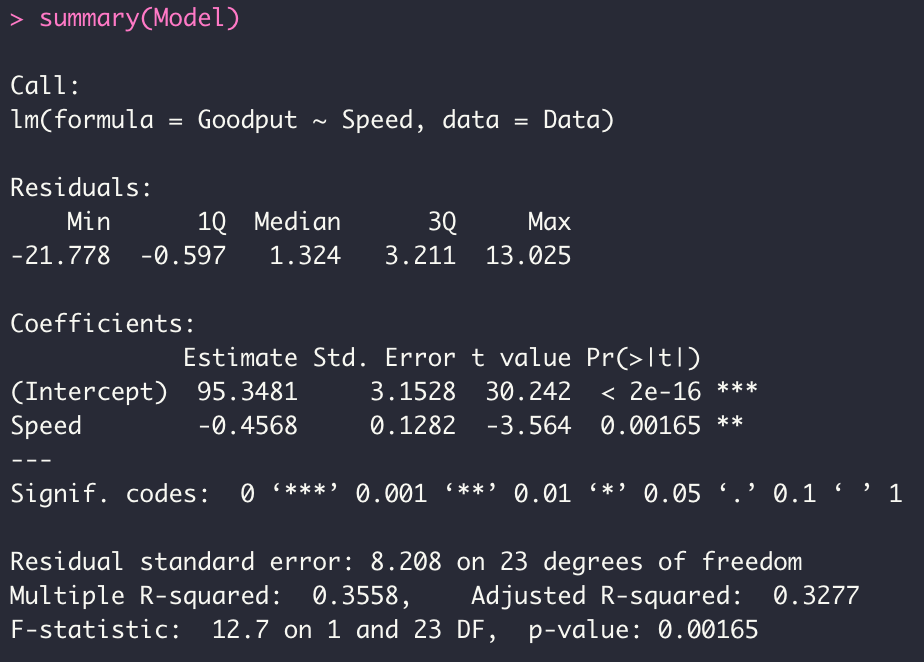
In the summary you see summary statistics about the residuals, followed by the estimated regression coefficients (Intercept $\hat{\beta}_0 = 95.3481$ and slope $\hat{\beta}_1 = -0.4568$ for the IV Speed), their standard errors ( $s_0 = 3.1528$ and $s_1 = 0.1282$ ), t-values when testing for a nonzero coefficient ( $t_0 = 95.3481/3.1528 = 30.242$ and $t_1 = -0.4568/0.1282 = -3.564$ ), and corresponding P-values (under $Pr(>|t|)$ ). The significance codes indicate how small the P-values are.

Then you have values for the Residual standard error (which is the square root of the $MSE$ , and is an estimate of $\sigma$ , in this case $8.208$ ) and its degrees of freedom, the $R^2$ (Multiple R-squared, in this case $0.3558$ ), and some additional information.

If you want to see the vector of the fitted values (the predictions of the dependent variable $\hat{y}_1 ,...,\hat{y}_n$ for each value of the independent variable based on the regression line, also called the "Y-hat" values) for this model, you would give the $\mathrm{R}$ command:

> Model$fitted.values

Similarly, if you want to display the vector of the residuals (the differences between observed and predicted values of the dependent variable) $e_1,...,e_n$ for this model, you would give the command:

> Model$residuals

To display the vector of coefficients (the beta-hats) $\hat{\beta}_0$ and $\hat{\beta}_1$ for the estimated regression function, you would give the command:

> Model$coefficients

Scatterplot

Suppose you want to make a scatterplot in $\mathrm{R}$ with the IV Speed on the horizontal axis and the DV Goodput on the vertical axis. The $\mathrm{R}$ command is:

> plot(Data$Speed, Data$Goodput)

The first argument to the $\mathtt{plot()}$ function is the column corresponding to the variable associated with the horizontal axis, which should always be the IV, and the second argument is the column corresponding to the variable associated with the vertical axis, which should always be DV.

The resulting scatterplot is inadequate. It has no title, and the axis labels aren't very informative. Also, the plotted points are open circles, while one might prefer dark filled-in circles. To fix this, we can add some additional settings to the $\mathtt{plot()}$ command:

> plot(Data$Speed, Data$Goodput, main="Computer Networks", xlab="Speed(M/s)", ylab="Goodput(%)", pch=20)

Now we obtain a much nicer scatterplot: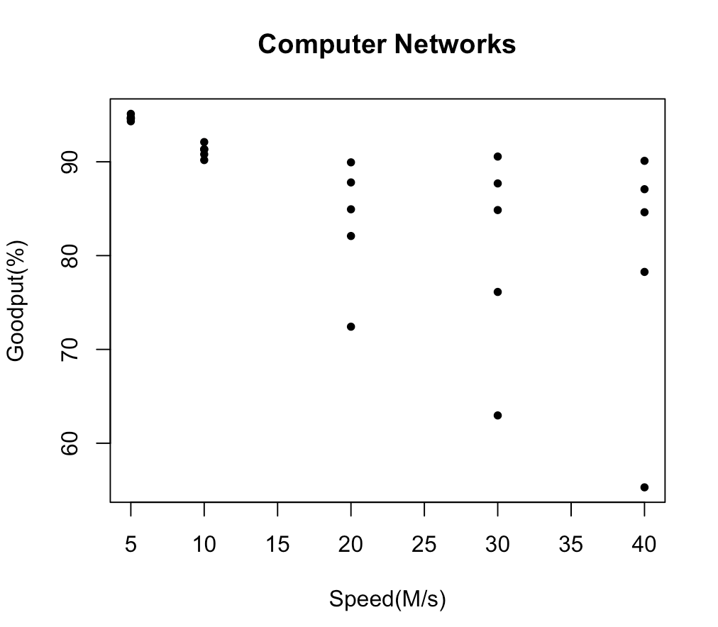You may want to also add a plot of the estimated regression line to the scatterplot of the data, since you have already obtained the least-squares estimates of the regression coefficients, which are stored in $\mathtt{Model$coefficients}$ .

To add the plot of the estimated regression function to the scatterplot, use the $\mathtt{abline()}$ command. This command takes the intercept of the line as its first argument, and the slope as the second argument.

> abline(Model$coefficients)

The line will appear superimposed over the data on the scatterplot: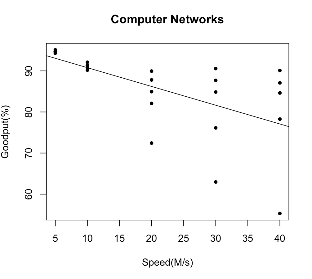

Confidence Intervals

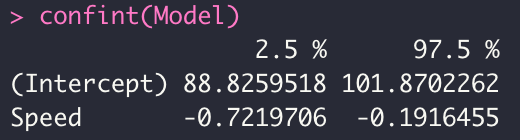
Let us return to our original model. To obtain $95\%$ confidence intervals for the intercept $\beta_0$ and the slope $\beta_1$ in the above linear model named Model, the $\mathrm{R}$ command would be:

> confint(Model)

Then $\mathrm{R}$ will display the lower bound and upper bound of the confidence interval for each parameter:

To obtain confidence intervals with another confidence level, say, $99\%$ confidence intervals, you would use:

> confint(Model, level=0.99)

Two-sided Hypothesis Testing

If you want to conduct the hypothesis test

$H_0 : \beta_1 = 0$ against $H_1 : \beta_1 \neq 0$

Notice that for the slope (after the word "Speed") under $\mathtt{t\,value}$ we have a t-value of $-3.564$ . This is just the estimated slope divided by its standard error.

The two-sided P-value is given to you under $\mathtt{Pr(>|t|)}$ , which in this case is $0.00165$ , and leads us to conclude in favor of $H_1$ at the $\alpha = 0.01$ level, i.e., Speed has a significant effect on Goodput. (Note: The summary will not display a P-value smaller than $2 \text{x} 10 ^{-16}$ , but will simply display $<2e\text{-}16$ , which is essentially zero.) The two stars in the last column of the summary tell you that the given P-value is between $0.001$ and $0.01$ (in the significance codes line).

You would test $H_0 : \beta_0 = 0$ against $H_1 : \beta_0 \neq 0$ in the same way. Note that in this example, the P-value for the intercept is $<2e\text{-}16$ (essentially zero), so you would also reject $H_0$ at any typical significance level.

One-sided Hypothesis Testing

If you have a one-sided alternative hypothesis, like $H_1 : \beta_1 > 0$ or $H_1 : \beta_1 < 0$ , you should divide the given two-sided P-value in half, but you must also make sure that the sign of the slope estimate is in agreement with the alternative hypothesis before you can conclude in its favor.

Test for a Nonzero Slope Coefficient

If you want to conduct a test in which the null value $\beta_{10}$ for the slope is not $0$ , you will have to divide the difference between the parameter estimate and the null value by the standard error to get the test statistic, i.e.,

$t_1 = \cfrac{\hat{\beta}_1 - \beta_{10}}{s_1}$ and then compute the P-value using the $\mathtt{pt()}$ function with $n - 2$ degrees of freedom. The procedure is similar for testing the intercept.

Coefficient of Determination

The value of the coefficient of determination $R^2$ is given in the original model output as $\mathtt{Multiple\,R}\text{-}\mathtt{Squared}$ . In this example it is $0.3558$ .

The value of $R^2$ is the proportion of the variation in the dependent variable that is explained by the association with the independent variable in the regression model, which we may re-format as $35.58\%$ .