The highest value of a part of a graph is called a
local maximum.
The lowest value of a part of a graph is called a
local minimum.
Both are extreme values of a function.
If we look at a function on a restricted domain, the values on the domain's boundaries can also be local maxima or minima and thus extreme values.
For example, we can view the function #f(x)=x^2# on the domain #\ivcc{2}{5}#. We now have a local minimum at #x=2# and a local maximum at #x=5#. When #x^2# is considered on its normal domain, there is only a local minimum at #x=0#.
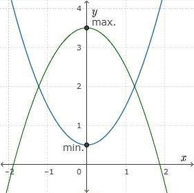
So far in this course, we have often specifically examined the #x# values of special points, but the maximums and minimums are the #y# values of these points.
Thus, in the example, a local maximum of the green graph is #3.5# and #\red{\text{not}}# #0#. A local minimum of the blue graph is #0.5# and #\red{\text{not}}# #0#.
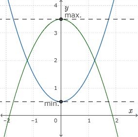
We have seen that the local maxima and minima are the highest points on a part of the graph. The global maximums and minimums are the highest points of the whole graph.
In the example of the green graph, the local maximum is also global. Similarly, in the blue graph, the local minimum is also global. This is not always the case.
Even if there are local maxima and minima, there may not always be a global maximum or minimum.
Using the derivative, we can easily calculate the extreme values of a function.
#\phantom{space}#
If a function #\blue{f(x)}# has a local maximum or minimum at #x=\orange{c}# then #\green{f'(\orange{c})}=0#.
If #\green{f'(\orange{c})}=0# and the graph of #\blue{f(x)}# changes from increasing to decreasing or vice versa at #x=\orange{c}#, then the function #\blue{f(x)}# has a local maximum or minimum at #x=\orange{c}#.
Example
\[\begin{array}{rcl}\blue{f(x)}&=&\blue{x^2}\\ \green{f'(x)}&=&\green{2x}\\ \green{f'(\orange{0})}&=&0\end{array}\]
The graph of #\blue{f(x)}# changes from decreasing to increasing at #x=\orange{0}#.
#\blue{f(x)}# has a minimum at #x=\orange{0}#.
The function must also be differentiable at the point #x=\orange{c}#. In this course, we will not look at functions that are not differentiable, but this can occur in practice.
If the derivative at a point equals zero, then the tangent line to the function is horizontal, as we can see in the picture.
This theorem does not hold if #c# is a boundary value of the domain on which the function is defined. For example, if we take #f(x)=x^2# on the domain #\ivcc{2}{5}#, then #2# and #5# are extreme values, but the derivative does not equal #0# in those points.
The first statement only holds one way. If the derivative #\green{f'(x)}# of a function #\blue{f(x)}# equals #0# in a point #\orange{c}#, it does not immediately mean that #\blue{f(x)}# has an extreme value in #\orange{c}#. It is necessary for the slope of the function to change direction at #\orange{c}# for the function to have an extreme value there (statement two).
Example
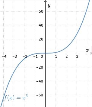
The derivative of #\blue{f(x)=x^3}# is equal to #0# at the point #x=\orange{0}#, but the function does obviously not have an extreme value at that point. The graph of #\blue{f(x)}# is increasing before and after #x=\orange{0}#.
| |
Step-by-step
|
Example
|
| |
Determine the extreme values of a function #f(x)#. Determine for each extreme value whether it is a local minimum, local maximum or neither.
|
#\qqquad \begin{array}{rcl}f(x)\phantom{'}&=&x^4-2x^2\end{array}#
|
| Step 1 |
Calculate the derivative #f'(x)#.
|
#\qqquad \begin{array}{rcl}f'(x)&=&4x^3-4x\end{array}#
|
| Step 2 |
Solve #f'(x)=0# to find the #x# coordinates of the points which are possibly an extreme value.
|
#\qqquad \begin{array}{rcl} 4x^3-4x&=&0\\ x=\green 0 &\lor& 4x^2-4=0\\ x= \green 0&\lor& x^2=1\\ x=\green{0} &\lor& x=\blue{-1} \lor x=\orange{1}\end{array}#
|
| Step 3 |
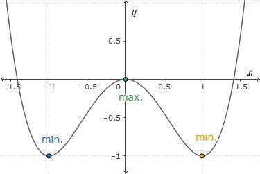
Sketch the graph to find out which points are a local maximum and which points are a local minimum (and which points may not be a maximum or minimum).
If sketching is difficult, do a sign chart analysis instead.
|
|
| Step 4 |
Substitute the obtained #x# coordinates in #f(x)# and determine the extreme values this way.
|
#f(\blue{-1})=-1#,
#f(\orange{1})=-1#,
#f(\green{0})=0#
Therefore, there are two local minima with value #-1# at #x= \blue{-1}# and #x=\orange{1}#, and a local maximum with value #0# at #x=\green{0}#.
|
Calculating the extrema of functions is something which appears often in optimisation problems. Problems are described by functions, whose minimum or maximum is determined.
We will give a very easy example. Suppose a farmer wants to fence a rectangular field, and he has bought #500# metres of fence. The farmer wants to maximise the fenced area, and wants to know the best ratio of the rectangle. We first note that this area #A# is given by #x\cdot y#, where #x# is the width and #y# is the depth of the rectangle. The farmer bought #500# metres of fence, which has to be distributed over the width and depth, which gives us #2x+2y=500#. Rearranging gives \[y=250-x\] We insert this in the function for the area and get \[A=x\cdot(250-x) = 250\cdot x - x^2\] This is the formula whose maximum we would like to calculate. Following the step-by-step approach, we get #x=125#. Thus, the farmer should fence a square area to maximise the area fenced.
In most applications, the functions are very complicated and contain many more variables. However, we will not be studying this in this course.
As an alternative to step #3#, sketching the graph, we can use a so-called sign chart or sign diagram. In step #2# we found the zeroes #x_1,\ldots, x_n# of the derivative #f'(x)#. By definition, there are no zeroes in the intervals #\ivoo{x_i}{x_{i+1}}#. This means that the values of #f'(x)# in such an interval are all positive or all negative. If we take one point in the interval and substitute it in #f'(x)#, we immediately know the sign of the interval: positive or negative. We now write the signs down for all the intervals in a sign chart
| Intervals of #x# |
#\ivoo{-\infty}{x_1}# |
#x_1# |
#\ivoo{x_1}{x_2}# |
#x_2# |
#\ldots# |
#x_n# |
#\ivoo{x_n}{\infty}# |
| Sign of #f'(x)# |
#+# or #-# |
#0# |
#+# or #-# |
#0# |
#\ldots# |
#0# |
#+# or #-# |
By analysing this sign chart, we can determine whether a zero #x_1# of #f'(x)# corresponds to a local maximum, minimum, or none. This is done by considering the signs of the intervals surrounding it, which are #\ivoo{x_{i-1}}{x_i}# and #\ivoo{x_i}{x_{i+1}}#. If #f'(x)# changes sign at a zero, #f(x)# has an extreme value at that zero.
- If the sign of #\ivoo{x_{i-1}}{x_i}# is positive and the sign of #\ivoo{x_i}{x_{i+1}}# is negative, then #x_i# corresponds to a local maximum.
- If the sign of #\ivoo{x_{i-1}}{x_i}# is negative and the sign of #\ivoo{x_i}{x_{i+1}}# is positive, then #x_i# corresponds to a local minimum.
- If the sign of #\ivoo{x_{i-1}}{x_i}# is positive and the sign of #\ivoo{x_i}{x_{i+1}}# is also positive, then #x_i# does not correspond to an extreme value.
- If the sign of #\ivoo{x_{i-1}}{x_i}# is negative and the sign of #\ivoo{x_i}{x_{i+1}}# is also negative, then #x_i# does not correspond to an extreme value.
Example
In the step-by-step example, we found the zeroes #x_1=-1, x_2=0# and #x_3=1#. To find the signs in the second, fourth, sixth, and eighth columns, we choose the following values:
- For the interval #\ivoo{-\infty}{-1}# we choose for example #x=-2#. We have #f'(-2)=4\cdot (-2)^3-4\cdot (-2)=-24#, which is negative, so we put a minus in the table.
- For the interval #\ivoo{-1}{0}# we choose for example #x=-\frac{1}{2}#. We have #f'\left(-\frac{1}{2}\right)= \frac{3}{2}#, which is positive, so we put a plus in the table.
- For the interval #\ivoo{0}{1}# we choose for example #x=\frac{1}{2}#. We have #f'\left(\frac{1}{2}\right)= -\frac{3}{2}#, which is negative, so we put a minus in the table.
- For the interval #\ivoo{1}{\infty}# we choose for example #x=2#. We have #f'(2)=24#, which is positive, so we put a plus in the table.
This yields the following sign chart.
| Intervals of #x# |
#\ivoo{-\infty}{-1}# |
#-1# |
#\ivoo{-1}{0}# |
#0# |
#\ivoo{0}{1}# |
#1# |
#\ivoo{1}{\infty}# |
| Sign of #f'(x)# |
#-# |
#0# |
#+# |
#0# |
#-# |
#0# |
#+# |
| Graph of #f# |
decreasing |
|
increasing |
|
decreasing |
|
increasing |
We see that both #x=-1# and #x=1# correspond to local minima, and that #x=0# corresponds to a local maximum.
Give the two values of #x# for which the function #f# given by \[f(x)=x^3-2x^2+x+4\] has an extreme value (a local minimum or local maximum).
The smaller value of #x# is indicated by #x_-# and the greater value by #x_+#. Write your answers as a simplified fraction.
#x_-=# #{{1}\over{3}}# and #x_+=# #1#
| Step 1 |
We determine the derivative of #f(x)=x^3-2x^2+x+4#. This is equal to:
\[f'(x)=3x^2-4x+1\] |
| Step 2 |
We determine the #x# coordinates of the potential extreme values by making the derivative equal to #0# by solving the equation.
\[\begin{array}{rcl}3x^2-4x+1&=&0 \\ &&\phantom{xxx}\blue{\text{the equation we need to solve}}\\
x=\dfrac{4-\sqrt{(-4)^2-4\cdot 3\cdot 1}}{2\cdot 3} &\lor& x=\dfrac{4+\sqrt{(-4)^2-4\cdot 3\cdot 1}}{2\cdot 3} \\ &&\phantom{xxx}\blue{\text{quadratic formula}}\\
x=\dfrac{4-\sqrt{4}}{6} &\lor& x=\dfrac{4+\sqrt{4}}{6} \\ &&\phantom{xxx}\blue{\text{simplified}}\\
x=\dfrac{4-2}{6} &\lor& x=\dfrac{4+2}{6} \\ &&\phantom{xxx}\blue{\text{simplified}}\\
x={{1}\over{3}} &\lor& x=1 \\ &&\phantom{xxx}\blue{\text{simplified}}\end{array}\] |
| Step 3 |
We draw the graph of #f(x)#.
Therefore, there is a local maximum at #x={{1}\over{3}}# and a local minimum at #x=1#. Hence, both obtained #x# values are part of an extreme value.
Therefore, #x_-={{1}\over{3}}# and #x_+=1# |


 Extreme values