Analysis of functions

Optimization: Optimal quantity

Analysis of functions

Let #f# be a function defined on a domain #I#.

A point #a# of #I# where all values #f(x)# of #x# in #I# are no higher than #f(a)#, is called a global maximum.
In the same manner, a point #b# of #I# where all values of #f(x)# for #x# in #I# are at least #f(b)#, is called a global minimum.

Hence, global maxima are local maxima, but in general not every local maximum is a global maximum. The same holds true for minima.

Different domains with the same function rule for #f# can result in different global maxima. For example, take a look at #f(x)=1-x^3#.

On the domain #I = \ivco{1}{\infty}# the global maximum lies on the edge: #x=1#.
On the domain #I = \ivco{0}{\infty}# the global maximum lies on the edge: #x=0#.
If we choose the entire number line as domain, then #f# has no global maximum.

In the previous paragraphs we have seen that you can determine if a function increases or decreases with the help of the derivative, and that a local extreme always is a stationary point, in which the derivative is #0#. With this we can find local extremes. How can you find global extremes?

With help of the named properties, you can analyse a function #f(x)#. This is done by executing the following 7 steps.

Calculate all zeros of #f(x)#.
Calculate the derivative function #f'(x)#.
Determine all stationary points of #f(x)# (this means: the zeros of #f'(x)#).
Calculate the function value #f(x)# in each stationary point #x#.
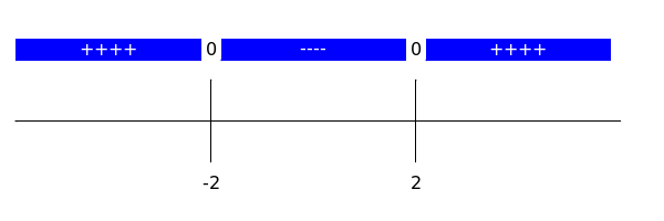
Create a sign diagram of # f'(x)#. This a diagram in which for values of #x# is indicated if the function #f(x)# increases (indicated by ++++) or decreases (indicated by ----). At stationary points the diagram contains a 0, since the derivative is equal to 0 at that point. This gives an indication of the intervals where the function is increasing/decreasing.
Create a precise drawing of the graph of the function #f(x)#.
Investigate whether the local maxima are also global maxima, as well as for local minima.

We will now take a look at an example where this procedure is executed.

Analyse the function \[f(x)=x^3-3\cdot x\]

The zeros of #f(x)# are #x=0 \lor x=\sqrt{3} \lor x=-\sqrt{3}#.
The derivative is #f'(x)=##3\cdot x^2-3#.
The stationary points of #f(x)# are #x=-1 \lor x=1#.
The corresponding extreme values are #f\left(-1\right)=# #2# and #f\left(1\right)=# #-2#.
The sign diagram of #f'(x)# looks like this:
The graph of #f(x)# looks like this:
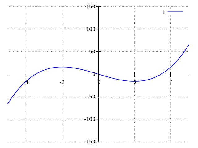
As for extreme points: at #x=-1# the function #f(x)# has a local maximum #2# and at #x=1# a local minimum #-2#. These local extrema are not global.

Re 1. First, we calculate the zeros of #f(x)#:
\[\begin{array}{rcll}
f(x) =0&&&\phantom{xx}\color{blue}{\text{the equation we have to solve }} \\
x^3-3\cdot x =0&&&\phantom{xx}\color{blue}{\text{function rule entered }} \\
x \cdot \left(x^2-3\right) =0&&&\phantom{xx}\color{blue}{\text{left hand side factored}} \\
x=0 \lor x^2-3=0&&&\phantom{xx}\color{blue}{A\cdot B^2=0\Leftrightarrow A=0\lor B=0} \\
x=0 \lor x=\sqrt{3} \lor x=-\sqrt{3}&&&\phantom{xx}\color{blue}{A^2=a\Leftrightarrow A=\sqrt{a} \lor A=-\sqrt{a}} \\
\end{array}\]

Re 2. Next, we calculate the derivative of #f(x)#. To this end we use the extended sum rule. It says that #f'(x)=\frac{\dd}{\dd x}\left(x^3\right)-3 \cdot\frac{\dd}{\dd x}\left (x\right)#.
With help of the polynomial rule for differentiation, which says that #\frac{\dd}{\dd x}\left(x^n\right)=n \cdot x^{n-1}# we now have:
\[\begin{array} {rcl} f'(x)&=&\frac{\dd}{\dd x}\left( x^3-3\cdot x\right)\\
&=&\frac{\dd}{\dd x}\left(x^3\right)-3 \cdot\frac{\dd}{\dd x}\left (x\right)\\
&&\phantom{xx}\color{blue}{\text{sum rule}}\\
&=&
3 \cdot x^{3-1} - 3 \cdot x^{1-1} \\
&&\phantom{xx}\color{blue}{\text{power rule}}\\
&=&3\cdot x^2-3 \end{array}\]

Now we calculate the stationary points of #f(x)#. Stationary points are the points for which we have #f'(x)=0#. Since #f'(x)=3\cdot x^2-3# we can find the stationary points the following way:
\[\begin{array}{rl}
3\cdot x^2-3=0&\phantom{xxx}\color{blue}{\text{equation entered}}\\
3\cdot x^2=3&\phantom{xxx}\color{blue}{-3 \text{ moved to the other side}}\\
x^2=1&\phantom{xxx}\color{blue}{\text{divided by 3}}\\
x=-1 \lor x=1&\phantom{xxx}\color{blue}{A^2=a\Leftrightarrow A=\sqrt{a} \lor A=-\sqrt{a}}\end{array}
\]

Re 3. Next we find the corresponding values of #f(x)# with the stationary points. We find the value of #f# at #x=-1# by entering #x=-1# in #f(x)#:
\[f\left(-1\right)=\left(-1\right)^3-3 \cdot \left(-1\right)=2\tiny.\]
We determine the value of #f# at #x=1# in the same manner:
\[f\left(1\right)=\left(1\right)^3-3 \cdot \left(1\right)=-2\tiny.\]

Re 4. Now we can make a sign diagram for #f(x)#. In the stationary points of #f#, we have #f'(x)=0#. Place the smallest stationary point on the left hand side, which is #-1# and the biggest one on the right, which is #1#.

Next you enter an #x \lt -1# in #f'(x)#. For example #x=-10#. Then you get #f'(-10)=3 \cdot (-10)^2 -3 =297#. Because #f'(x) \gt 0#, #f(x)# increases on the interval #x \lt -1# and you write down ++++.
Next you enter a #-1 \lt x \lt 1# in #f'(x)#. For example #x=0#. Then you get #f'(0)=3 \cdot (0)^2 -3 =-3#. Because #f'(x) \lt 0#, #f(x)# decreases on the interval #-1 \lt x \lt 1# and you write down ----.
Next you enter an #x \gt 1# in #f'(x)#. For example #x=10#. Then you get #f'(10)=3 \cdot (10)^2 - 3 =297#. Because #f'(x) \gt 0#, #f(x)# increases on the interval #x \gt 1# and you write down ++++.

This leads to the following sign diagram:

Re 5. If you take a look at the sign diagram of #f#, you see it has plus signs at the left up to #-1# and from #1# till the end. Hence, on the intervals #\ivoo{-\infty}{-1}# and #\ivoo{1}{\infty}#, the function #f# is increasing. On the part between #-1# and #1# the diagram has minuses, hence, on the interval #\ivoo{-1}{1}#, the function #f# is decreasing. This means that #\ivoo{-\infty}{-1}# and #\ivoo{1}{\infty}# are the increasing intervals of #f(x)#; the decreasing interval is #\ivoo{-1}{1}#.

Re 6. With this information, the graph of #f(x)# can be drawn. It is shown near the top of this solution.

Re 7. In addition, you can now identify the extreme points: at #x=-1# the function #f(x)# has a local maximum #2# and at #x=1# a local minimum #-2#. These local extrema are not global.

New example